
Abstract
The relationship between urban form and greenhouse gas (GHG) emissions has been studied extensively during the last two decades. The prevailing paradigm arising from these studies is that a dense or compact urban form would best enable low-carbon living. However, the vast majority of these studies have actually concentrated on transportation and/or housing energy, whereas a growing number of studies argue that the GHG implications of other consumption should be taken into account and the relationships evaluated. With this two-part study of four different area types in Finland we illustrate the importance of including all the consumption activities into the GHG assessment. Furthermore, we add to the discussion the idea that consumption choices, or lifestyles, and the resulting GHGs are not just a product of the values of individuals but actually tied to the form of the surrounding urbanization: that is, lifestyles are situated. In part I (Heinonen et al 2013 Environ. Res. Lett. 8 025003) we looked into this situation in Finland, showing how the residents of the most urbanized areas bring about the highest GHG emissions due to their higher consumption volumes and the economies-of-scale advantages in the less urbanized areas. In part II here, we concentrate only on the middle-income segment and look for differences in the lifestyles when the budget constraints are equal. Here we also add the variables housing type and motorization into the assessment. The same time-use and private expenditure data as in part I and the same GHG assessment method are used here to maintain high transparency and comparability between the two parts. The results of the study imply that larger family sizes and economies-of-scale effects in the less dense areas offset the advantages of more dense living when the emissions are assessed on per capita basis. Also, at equal income levels the carbon footprints vary surprisingly little due to complementary effects of the majority of low-carbon lifestyle choices. Motorization was still found to increase the emissions, but a similar pattern regarding housing type was not found.
Export citation and abstract BibTeX RIS

Content from this work may be used under the terms of the Creative Commons Attribution 3.0 licence. Any further distribution of this work must maintain attribution to the author(s) and the title of the work, journal citation and DOI.
1. Introduction
As the evidence for greenhouse gases (GHGs) warming the globe and for us humans bearing the responsibility accumulates (Cook et al 2013), the impact of the urban form on the emissions from a certain area has become a topic discussed with enthusiasm in recent years (e.g. Naess 2006, Marshall 2008, Jenks and Burgess 2000, Satterthwaite 2008). The prevailing paradigm arising from these and a multitude of other studies is that a dense or compact urban form would best enable low-carbon living.
The focus of the majority of the studies on the urban form–GHG-connections has been on traffic- and housing-related emissions due to the two being the largest contributors and the emissions being relatively easily accountable. In particular, traffic-related emissions have been found to decrease as the compactness of the urban form increases (Ewing and Cervero 2010, Bento et al 2005, Newman and Kenworthy 1989, 1999), but lower housing-energy use figures have also been reported when cities have been compared to their surrounding areas (Parshall et al 2010, Glaeser and Kahn 2010).
More compact urban forms have also been tied to lower per capita emissions compared to the surrounding areas or the country average (Stephan et al 2013, Fuller and Crawford 2011, Brown et al 2009, Dodman 2009, Hoornweg et al 2011, VandeWeghe and Kennedy 2007). This seems to hold in developed countries especially when the accounting method is territorially restricted accounting of the Kyoto Protocol type where the emissions are allocated based on the actual location of the emitter (known as producer responsibility allocation (e.g. Satterthwaite 2008)). However, the significant impact of affluence and consumption choices has been highlighted in several recent studies (e.g. Baiocchi et al 2010, Newman 2006, Minx et al 2013). More and more evidence implies that when the allocation method is user activity based 'consumer responsibility' (e.g. Lenzen et al 2007), the emissions caused by the often more affluent city resident may exceed the country averages (Lenzen et al 2004, Sovacool and Brown 2010, Heinonen 2012). Furthermore, these studies strongly suggest that it is not sufficient to look only at the emissions from transport and/or housing energy in the search for more sustainable urban forms.
With this two-part study we add to this discussion the idea that consumption choices, or lifestyles, and the resulting GHGs are not just a product of the values of individuals but actually strongly tied to the form of the surrounding urbanization, that is, lifestyles are situated (Heinonen et al 2013). The idea brought up earlier by e.g. Baiocchi et al (2010) has been studied relatively little. In part I we looked into this situation in Finland on a highly aggregated level and showed that, in a setting of the country divided into four different types of urban forms based on their level-of-urbanization (metropolitan, city, semi-urban and rural), the residents of the most urbanized areas cause the highest GHG emissions. Analyzing the purchasing and time-use patterns concurrently, we showed how the residents of the different types of areas share some lifestyle patterns that can be used to explain the differences in the emissions. Life in the less urbanized areas is significantly more home-centered, whereas the residents in the more urbanized areas spend their leisure time in service spaces where various consumption activities take place. We brought up the concept of parallel consumption to explain how the reduced living spaces in the more urbanized areas are actually a trade-off between living space possessed and high proximity to various service spaces that can be used to 'extend' the living space.
In part I, we also discussed one of the well-known effects of urbanization, namely, that cities create wealth and consumption opportunities for their residents, which lead to their residents having the highest carbon footprints. However, the notion of situated lifestyles calls and makes room for more varied effects that may also have important policy implications. In this letter, we thus concentrate on the middle-income segment and look for differences in the lifestyles when the budget constraint is equal. This opens up new understanding of the more direct effects of urban structure on consumption and of the ways that physical structures affect lifestyles. In addition, despite being able to show some significant differences in the lifestyles of the residents of the four area types in part I, it is evident that there are important factors affecting the GHGs within each area type, which should be analyzed further.
With this in mind, here in part II we employ housing type and the possession of cars, or motorization, as background variables that determine the lifestyles within each area type. These variables enable us to analyze a step further the GHG differences within as well as across the different area types. The same time-use and private expenditure data as in part I and the same GHG assessment method to maintain high transparency and comparability between the two parts are employed here.
In contrast to the findings in part I, we find that the emissions decrease slightly towards the more urbanized areas. However, for the studied middle-income segment, the differences in the GHG emissions are very small compared to those found in part I, and predominantly remain so throughout the analyzed variables. At an equal income level, the different lifestyles in different urban forms seem to lead to relatively similar GHG outcome even if there are significant differences in the structure of consumption expenditures and time allocation. One important explanation, which significantly reduces the GHG impact of any change in the consumption patterns, is that the consumption choices are mostly trade-offs between two consumption categories. Bearing that in mind, we find some variations between the area types especially due to the household sizes and the resulting economies-of-scale effect. Within the area types, motorization seems to increase the overall emissions somewhat, but housing type (high-rise–low-rise) does not seem to cause any clear differences.
In this part, the research design is explained in section 2. Section 3 presents the results, and in section 4 the findings are discussed further. The key conclusions of the two-part study are summarized in section 5.
2. Research design
This part II is a direct continuation of part I and employs the same data (Household Budget Survey 2006 and Time-Use Survey 2009–2010) and the same level-of-urbanization based division of the Finnish municipalities into four categories: Helsinki metropolitan area (HMA), other cities, semi-urban areas and rural areas. We also continue with the same input–output life cycle assessment (IO LCA) method in assessing the GHGs and maintain the per capita functional unit utilized in part I. These are all explained in detail in part I of the study.
For this part II, we take a step further to analyze how some of the key lifestyle variables affect the results within each area type and to describe how the lifestyles vary regarding Time-use and expenditure patterns along with the selected variables of motorization and housing. Firstly, we restricted our analysis on the middle-income segment by sampling out the per capita income deciles 5–7 from the Finnish income distribution. With this selection, the average in each area type falls between 16 600 € and 16 900 €,4 which is very close to the Finnish average disposable income 16 700 € per capita according to the Finnish Household Budget Survey 2006.
After this we divided the samples of the expenditure data and Time-use data further into subcategories within each of the four types of areas, according to the type of housing and possession of private cars (motorization). For the type of housing, we use a two-category grouping of low-rise (detached, semi-detached and terraced houses) and high-rise (apartment buildings). Motorization is similarly divided into two subgroups of no private cars in possession of the household (non-motorized) and one or more cars in possession of the household (motorized). In all the subgroups, the average disposable income is within the same range of 16 600–16 900 € /a. Figure 1 depicts the variables and the generated subcategories.
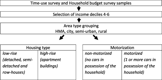
Figure 1. The sampling process and the utilized groupings.
Download figure:
Standard image High-resolution imageBoth the expenditure and the Time-use data were employed simultaneously to show how the lifestyles differ and which activities explain the GHG emissions. Rural areas were left out from the subgroup analyses of housing type and motorization due to high-rise and non-motorized lifestyles being too rare in the area type to be studied with the employed data. Finnish average GHGs are also shown for comparison benchmarks.
In part I, we showed a very detailed distribution of monetary expenditures, GHGs and Time-use. We also explained the GHGs with selected Time-use sectors. Here we utilize a more aggregated distribution of money, time and GHGs to take a step further in the concurrent analysis, which shows how the lifestyles vary and explain the GHGs. The categories are listed in table 1. The first six categories describe spaces, the related expenditure, GHGs and time that is allocated for various uses of these spaces. The categories 7 and 8 lines are not spatial categories but rather describe functions, related GHGs and Time-use. Categories 9 and 10 do not have direct equivalents in expenditures or GHGs, but have a role in the lifestyle analysis as is shown later in the letter.
Table 1. The categorization of the expenditure and Time-use data.
| Expenditures and GHGs | Time-use | |
|---|---|---|
| 1 | Primary home | Domestic activities |
| 2 | — | Outdoor recreation |
| 3 | Second homes | Second homes |
| 4 | Services | Services |
| 5 | Ground transport | Ground transport |
| 6 | Traveling abroad | Long distance travel |
| 7 | Food at home | Food at home |
| 8 | Tangible goods | Shopping |
| 9 | — | Work and school |
| 10 | — | Sleeping and resting |
'Primary home' includes construction, operation and maintenance of buildings, housing energy being the largest single sector. From the Time-use perspective, the 'Domestic activities', the time spent at home minus sleeping and food-related activities, describes the activities for which the homes provide. In addition, 'Outdoor recreation' encompasses the natural and built public outdoor environment. 'Second homes' comprises the same expenditure and GHG sectors as 'Primary home' but related to other possessed living spaces including cottages, and in 'Time-use' the time spent at these premises. 'Ground transport' combines the expenditures on and the GHGs from purchases and operation of private vehicles and utilization of public transport and taxis, and the time spent in traffic using these vehicles. 'Services' depicts the expenditure on and the GHGs from a large variety of services, dominated by leisure services like hotels, restaurants and cultural services, and the time spent consuming these. 'Traveling abroad' includes flights, ferries and package holidays, but the expenditures abroad as well, whereas 'Long distance travel' depicts the time spent traveling to locations abroad. 'Food at home' includes all the groceries and drinks consumed at home, that is, cooking and eating at home. 'Tangible goods' comprises all the purchases of tangible goods outside of the earlier sectors. Different appliances and sports goods form the largest sectors, but their distribution is wide. There is not a good equivalent for this consumption in 'Time-use', but 'Shopping' time shows if the differences in purchases are reflected to time spent in shopping. The first six spatial categories reflect the most the parallel consumption of different service spaces that we proposed in part I.
3. The lifestyles and the resulting GHGs in the four area types
3.1. The middle-income segment
With only the middle-income segment included in the analysis, the variation between the studied four area types is reduced to a fraction of what we reported in part I. In contrast to part I results, the residents in HMA would now seem to cause slightly less GHG emissions than the residents of the less urbanized areas. In HMA, the carbon footprints are approximately 9600 kg CO2e/a, increasing to 10 000 kg CO2e/a in cities and in semi-urban areas and up to 10 300 kg CO2e/a in rural areas. In addition, the GHG intensity of consumption seems to be lower in HMA, where the annual expenditure is higher and savings rate lower than in the other area types. The intensity is approximately 0.6 kg CO2e/€ in HMA, whereas in the three other area types the respective figure is 0.7 kg CO2e/€.
Even at equalized income levels there seems to be lifestyle differences similar to those we reported in part I. Differences in the emissions from utilization of private vehicles fully explain the above differences in GHGs and actually even exceed them. However, even at equal income levels there seems to be more personal consumption in the more urbanized areas (see part I for a detailed discussion). According to the parallel consumption hypothesis set out in part I, more money and time are allocated to consumption of services in the more urbanized areas. This closes down the gap in the GHGs, but not enough to fully absorb the benefits from transport. Purchases of tangible goods also increase towards the more urbanized areas, especially lifestyle goods like clothes and footwear, and services such as restaurants and cultural events, belong to categories where the differences remain significant despite the equalized income level.
'Services' are actually a controversial category from the GHG perspective. In comparison to the money allocated to services, the amount of emissions is not very high, but the emissions are actually a result of relatively little Time-use; service-time is energy intensive and, furthermore, time-saving services result in a Time-use rebound effect as new opportunities for working and consuming are available (Jalas 2002). Services also indicate parallel consumption, since many of them can be considered as extensions of the possessed living space, but using them does not necessarily reduce the housing-related emissions.
Interestingly, no clear pattern in the emissions from the primary home can be found. It is the largest single sector contributing to GHG emissions in all the area types, but the differences between the areas are small. Furthermore, the HMA residents spend the most money on their home, but allocate the least time for staying at home.
Second homes and cottages do not seem to cause much emissions, but it is well-known that private driving is the predominant mode of transport in traveling to cottages (Perrels and Kangas 2007). Therefore, the ownership of cottages in the more urbanized areas may actually increase the emissions from ground transport as well.
Food at home causes rather similar emissions in all the area types, though slightly less in the more urbanized areas, reflecting the more frequent eating out there. Traveling abroad causes little emissions in overall but slightly more in the more urbanized areas, especially in HMA, which agrees with the lifestyle differences found in part I. However, in contrast to what we reported in part I and what some previous authors have suggested (Ornetzeder et al 2008, Holden and Norland 2005), increased air travel of city dwellers seems not to undo the benefits of denser living in an income neutral situation. Figures 1(A)–(C) depict these differences in the lifestyles from the perspective of money and time allocation and the resulting GHGs.
3.2. The impacts of housing type and motorization on the GHGs
Adding the variables housing type and motorization into the assessment spreads the between-sample differences surprisingly little, as table 2 shows. Motorization seems to lead systematically to somewhat higher emissions in all area types, the non-motorized lifestyle performing between 300 and 700 kg CO2e/a better in comparison to the motorized subgroup. Surprisingly, housing type does not seem to have a similar clear pattern. With equal disposable income, the high-rise and low-rise residents cause a very similar amount of emissions in the more urbanized areas. In semi-urban areas, the high-rise residents actually cause clearly more emissions than the low-rise residents, the approximate difference being 1500 kg CO2e/a.
Table 2. The average annual carbon footprints in the different subgroups (kg CO2e/a).
| Overall | Motorized | Non-motorized | High-rise | Low-rise | |
|---|---|---|---|---|---|
| Finland | 10 030 | 10 160 | 9 390 | 10 000 | 10 030 |
| HMA | 9 610 | 9 830 | 9 200 | 9 650 | 9 550 |
| City | 10 000 | 10 130 | 9 450 | 9 850 | 10 110 |
| Semi-urban | 10 000 | 10 010 | 9 770 | 11 350 | 9 820 |
| Rural | 10 330 | 10 460 | n.a. | n.a. | 10 180 |
Two key factors were identified to explain why the differences in the overall GHGs are relatively small between the subgroups. Firstly, at equal income levels the consumption choices are mostly trade-offs between allocation of time and money to one type of consumption and some other. Due to this trade-off, or rebound effect, any reductions in the GHGs tend to be compensated to a significant extent by the emissions from the activity where the time and money are re-allocated.
Because we assess the emissions on the per capita level, the second factor significantly affecting the results is the average household size, which varies significantly between the subgroups. Non-motorized lifestyle seems to associate strongly with being single or at least childless, whereas motorization increases significantly along with the household size. In each area, the average household size roughly doubles in the motorized subgroup in comparison to the no-cars group. This means that the emissions from housing especially, but also from many other goods, are attributable to a very different number of people in the different subsamples. Regarding housing, the non-motorized have on average 8–13 m2 per capita more living space in each area type, due to the very small household sizes according to the employed input data.
Similarly, the household size largely explains why high-rise living cannot reduce per capita emissions when comparing the high-rise and low-rise residents. The difference is not as large as in motorization, but at the household level the economies-of-scale effect is strong enough to even out the GHGs since the emissions from especially housing are attributable to fewer persons in the high-rise households. The differences in the household sizes lead to the high-rise subgroup having on average only 5–8 m2 less living space per capita in each area type in comparison to the low-rise group. And since in high-rise buildings there are large communal spaces, the actual space for housing might be even higher in the high-rise group. Table 3 shows the average household sizes.
Table 3. The average household sizes and the living spaces per capita (m2/capita) in the different subgroups.
| Non-motorized | Motorized | High-rise | Low-rise | |||||
|---|---|---|---|---|---|---|---|---|
| Household size | Living space | Household size | Living space | Household size | Living space | Household size | Living space | |
| HMA | 1.4 | 41.2 | 2.6 | 31.6 | 1.8 | 33.3 | 2.6 | 37.9 |
| City | 1.2 | 49.3 | 2.3 | 41.3 | 1.5 | 39.0 | 2.5 | 45.3 |
| Semi-urban | 1.1 | 61.7 | 2.4 | 48.3 | 1.4 | 42.4 | 2.4 | 50.2 |
It would also seem that expensive housing has only a moderate positive rebound effect even when the disposable income is equal (i.e. leading to less other consumption). In HMA, the housing prices are significantly higher than in the rest of the country, but instead of having less other consumption at an equal level of disposable income, the average HMA resident has a low personal savings rate. High expenditure on housing could reduce other consumption even up to a level where the overall emissions would decrease, but in this example the HMA residents are not giving up on other consumption, just reducing their saving. The average resident of HMA actually ends up with a higher overall expenditure level in all the subgroups when comparing the different types of areas (table 2 shows this in the groups of non-motorized and motorized). The impact of higher housing prices in HMA has been removed from the GHG assessment regarding the emissions from housing (see part I for a detailed description), but the monetary analysis shows how the high price level in housing shows as increased overall consumption.
3.2.1. High-rise and low-rise lifestyles.
Even though the overall GHG emissions of high-rise and low-rise lifestyles are relatively similar, notable differences can be observed in their disaggregated GHG emissions profiles. Figures 3(A) and (B) below depict the variation of the GHGs between the high-rise and the low-rise residents and how the allocation of time changes within the employed distribution (see section 2 for the category definitions). Figure 3(A) shows how the economies-of-scale in the housing-related emissions is a relatively strong factor in explaining the GHGs. In contrast to what has been reported in many earlier studies, the housing-related emissions are either equal or higher in the high-rise group when compared to the low-rise group within each area type on a per capita basis. In semi-urban areas, the very small average household size in the high-rise group shows as high emissions from housing but also as very high emissions from transport since nearly all the emissions are attributable to a single person. From the per capita perspective, the high-rise residents actually seem to cause similar or even higher emissions from transport in each area type.
Surprisingly, the high-rise residents spend slightly more time at their smaller and more urban homes. However, the active time at home is very similar between the housing types in HMA and in cities and clearly different only in semi-urban areas. The low-rise residents allocate more time to work and school but cover up the difference in active leisure time by sleeping less. In HMA, the difference in the average daily sleeping time is, strikingly, almost an hour per day. Combined with the fact that the high-rise residents also watch on average 30 minutes more TV, domestic time in low-rise buildings is far more active.
3.2.2. Non-motorized and motorized lifestyles.
When turning to a deeper analysis of motorization, the differences in the lifestyles are actually more visible in GHGs as well as in time. Firstly, it seems that private driving is an activity where reduced expenditure is not fully re-allocated elsewhere; the overall expenditures of the motorized are systematically higher in comparison to those of the non-motorized. Thus the motorized households spend a larger share of their disposable income and use a significant share of this in rather GHG-intensive private driving. Increased use of public transport of the non-motorized increase their transport-related expenditures and the GHGs, but only to a very limited extent. Table 4 compares the transport-related and the overall consumption of the non-motorized and the motorized5.
Table 4. The average monetary expenditures (€/a) of the no-cars group and the motorized on transport and the overall annual expenditures among the middle-income segment.
| HMA | City | Semi-urban | ||||
|---|---|---|---|---|---|---|
| No-cars | Motorized | No-cars | Motorized | No-cars | Motorized | |
| Acquisition and use of private vehicles | 170 | 2 590 | 370 | 2 060 | 340 | 2 020 |
| Public transport | 550 | 190 | 360 | 120 | 180 | 60 |
| Overall consumption expenditure | 14 730 | 16 550 | 13 370 | 14 830 | 13 450 | 14 470 |
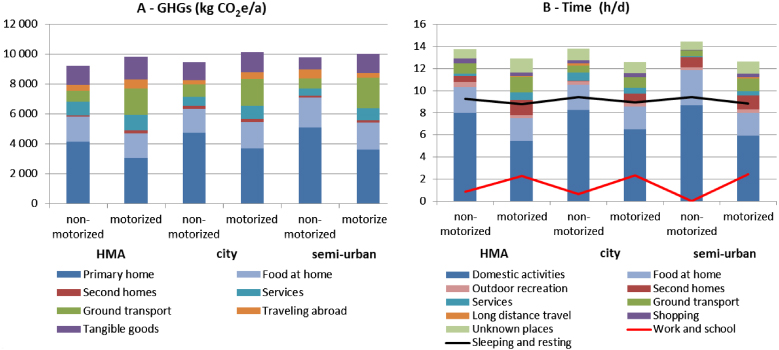
Secondly, very similarly to the previous housing type analysis, the small household size of the non-motorized has an opposite impact on the GHGs. The single households are predominantly non-motorized, their emissions, from housing especially, being attributable almost fully to a single person. The motorized households create more transport-related GHGs than expected, but interestingly almost fully offset this difference in lower housing emissions due to the economies-of-scale effect as a consequence of the larger household size, as figure 4(A) depicts. It is also interesting that the motorized cause very similar emissions from transport in all the area types. Thus, the overall lower GHGs from ground transport in the more urbanized areas (see figure 2) result from a higher share of the carless residents, but those who possess cars have relatively equal trip generations in all the area types.
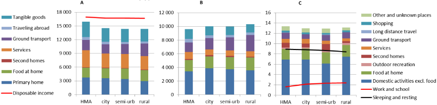
Figure 2. The annual per capita (A) disposable income and expenditure (€ /a), (B) GHGs (kg CO2e/a) and (C) time allocation (h d−1) in the four area types.
Download figure:
Standard image High-resolution image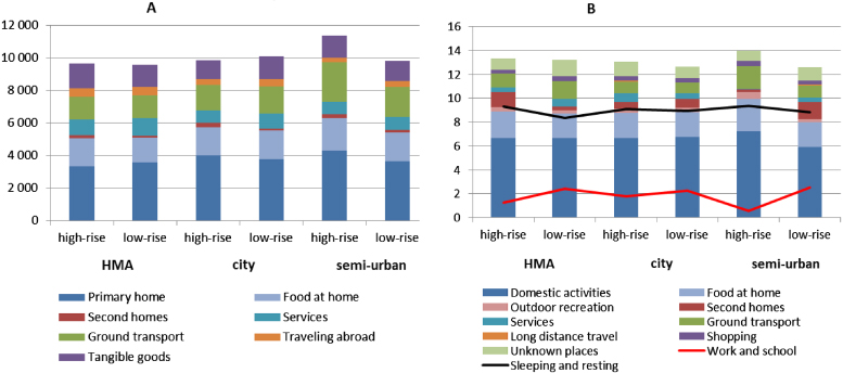
Figure 3. The average per capita (A) GHGs (kg CO2e/a) and (B) time allocation (h d−1) in the high-rise and low-rise subgroups in the different area types.
Download figure:
Standard image High-resolution imageFurthermore, the small household sizes of the non-motorized seem to lead to them being required to work considerably less to reach the selected per capita income level. As a result, the non-motorized have more leisure time. Still it seems that motorization especially prompts activities outside of home, or parallel consumption, such as the use of the second homes and services as figures 4(A) and (B) depict. Despite better availability of services at close proximity, motorization, even in HMA, relates to higher use of services revealing how many consumption activities take place outside the immediate living neighborhood requiring private vehicles. On the other hand, the non-motorized seem to have more home-centered lifestyles, which also restrain the emissions they cause. Across all the area types, they spend the majority of the excess leisure hours at home: sleeping, resting, reading or watching television. The home-centered lifestyle of the non-motorized people shows also in a clear increase in the time spent on meals and food-related activities.
Figure 4. The average per capita (A) GHGs (kg CO2e/a) and (B) time allocation (h d−1) in the non-motorized and motorized subgroups in the different area types.
Download figure:
Standard image High-resolution image
The differences in the time spent at home are rather large. In cities, the average time spent at home is 18.5 h d−1 for the non-motorized and 16.3 h d−1 for those with a car, and in semi-urban areas the respective figures are 20.9 h d−1 and 15.9 h d−1. The effects of motorization are thus amplified in the less dense areas. Notwithstanding, density also prompts residents towards parallel consumption: time spent at home is the shortest in the HMA for both carless and motorized people across the different area types.
4. Discussion
This study was set to analyze the impact of the spatial location on the GHG emissions of the consumption activities. The premises were presented in the part I, where we showed that the average GHG emissions increase towards the more urbanized areas due to higher overall consumption and the economies-of-scale effect in the less urbanized areas. In this part II, we narrowed the sample to only the middle-income segment in Finland and looked for differences in the lifestyles when the housing types and the level of motorization change within the same area types as in part I.
We found that in overall the differences in the carbon footprints are relatively small at an equal income level, but also some interesting differences were found. Firstly, and in contrast to the results of part I, the GHGs caused by the middle-income segment seem to be slightly lower in HMA when compared to the other three area types, but the variation is low. Secondly, when calculating on a per capita basis, no support can be found for the prevailing belief that high-rise living would be more GHG efficient in comparison to low-rise living in the current situation in Finland. According to the study, the low-rise residents actually cause equal or lower overall emissions. Their larger family sizes increase rapidly the economies-of-scale effect, especially regarding the housing-related emissions, but also as far as the emissions from many other shareable goods are concerned. However, these gains in efficiency are currently largely compensated elsewhere as the larger family sizes relate strongly to low-rise living and use of private vehicles. This notion gives arise to a need to study further the differences of similar family types living in different types of apartments.
Motorization was found to be related to higher GHG emissions within each area type. However, due to the economies-of-scale effect the gains of the non-motorized in the transport-related emissions are largely lost due to high housing-related emissions. Still, the availability of cars seems to be the strongest driver of parallel consumption (the consumption of other living and service spaces in addition to an equipped home as defined in part I), which increases the emissions of the motorized to a higher level than those of the non-motorized in all the area types. Among the middle-income segment, parallel consumption is not as clearly a character of urban living as that set forth in part I, but across the area types the HMA residents spend the most time in various service and living spaces outside their own residence and increase their climate impact.
One result of the study, rather obvious when analyzing a narrow income group but affecting the GHGs significantly, is the rebound effect. Money saved on one issue opens up consumption possibilities elsewhere, and this re-allocation of consumption significantly reduces the GHG effects of giving up on even some GHG-intensive activity. For example, Hertwich (2005) has discussed the importance of paying attention to this effect when the sustainability of consumption is addressed. However, we also found that saving rates differ in the different lifestyle groups analyzed in this study: high expenditure on housing and private driving are not fully compensated by reduced expenditure on other consumption but show as high an overall expenditure level even at equal income. Especially in private driving this effect adds to the GHG contribution of the motorized life styles in all the area types.
Overall, we have demonstrated in this part II study that even at an equal income level the lifestyles and thus the resulting GHG emissions are always affected by the qualities of the spatial location where one resides, being thus situated lifestyles. Inevitably there are significant variations within each subgroup of our study, but even on a relatively highly aggregated level the lifestyles within each group seem to have common components explained by the surrounding urban form.
Our results comply relatively well with the earlier literature on the GHGs from different types of urban structures where some kind of income control has been employed. e.g. Herendeen and Tanaka (1976), Lenzen et al (2006) and Shammin et al (2010) suggest that, when studying dwellers in different spatial locations with the wealth level controlled, the more urban tend to cause approximately 10% less emissions. Druckman and Jackson (2009) reported that when the per capita level average emissions are compared, countryside living would be slightly less carbon intense than life in prospering suburbs. However, the differences in the wealth levels are not explicitly controlled in their study.
In our study, we chose to cut away the low- and high-income residents and concentrate on the middle-income segment. The method of income level standardization more often utilized has been regression analysis (Herendeen and Tanaka 1976, Shammin et al 2010). Regression analysis is a more refined way to predict or explain the variable of interest. However, comparing means with standardized income levels offers also informative insights and reduces some of the inherent weaknesses of the employed GHG assessment method as well (see below for further analysis).
It would be interesting to examine how controlling the amount of work as well would affect the results. Income affects the lifestyles significantly, but time restrictions put another type of pressure on the consumption choices. Within the middle-income segment there are significant differences in the average amount of work between different groups, which inevitably affect their lifestyles. Similarly, controlling age in a future study would be interesting, since it is probably another factor that affects the lifestyles significantly. More broadly, positing income and hours of paid work as lifestyle choices would connect discussions concerning urban structure to existing literature on downshifting and de-growth (Sanches 2005, Schor 2005, Nørgård 2013).
The carbon footprint assessments in the study utilize a streamlined LCA in the sense that only GHG emissions are accounted for (Crawford 2011). Currently, climate change is in the nexus of environmental concerns, but other impacts such as biodiversity, toxicity and resource depletion already are or soon may become as important. e.g. Rockström et al (2009) suggest that 'humanity has already transgressed three planetary boundaries: for climate change, rate of biodiversity loss, and changes to the global nitrogen cycle'. According to Laurent et al (2012), GHGs do not properly indicate other environmental impacts and GHG mitigation actions may even increase other impacts. Thus in the future the other connections between lifestyles and environmental impact should be studied further.
Another limitation of the study is that we chose to utilize the average emissions intensities of Finland's energy production for all the studied samples. We took into account the variations in the heating modes, but not the spatial or plant-based variation in the energy mix, i.e. the fuels used in specific energy production plant within a certain region. Taking these into account would actually lead to much larger variation in the results than what we found now. For example, Heinonen and Junnila (2011) have demonstrated how production, in a certain location, based on renewable fuels can significantly reduce the per capita GHGs in the Finnish context, where fossil fuels have a major role in combined heat and power production (Finnish Energy Industries 2012).
Fuels and delivery networks for large-scale energy production could provide a significant potential for centralized transformation towards less carbon intensive living; if the fuel-mix changes, it automatically affects the GHG emissions on a large scale. The challenge is the complex decision-making structure, and thus this is not so much of a lifestyle issue. In the case of detached housing, the situation is different. The individuals can quite independently choose to use low-carbon technologies such as heat pumps and fireplaces for heating purposes, which could considerably reduce the reported average emissions. All of these options are actually already being more and more widely used, which could also partially explain the relatively good performance of the low-rise residents regarding housing-related emissions. According to the statistics of the Finnish Forest Institute METLA, an average household living in a detached house in Finland burns an average of 3.2 m3 of firewood a year (Torvelainen 2009), which is equivalent to over 20% of the overall energy use of a household in kilowatt hours.
The study suffers from some other deficiencies and uncertainties as well. The potential biases related to the input data are basically the same as in part I, and thus a detailed discussion on them can be found from there. The risk of data biases due to small sample sizes is more severe in this part II since the same samples were divided further to subsamples. To avoid this problem, we left the rural area type out from the housing type and motorization subgroupings since there were only very few observations in the data in these groups. In HMA, city and semi-urban subsamples, the sample sizes number approximately 50 or over in all but two subsamples in both expenditure and time-use data. The high-rise and the non-motorized subsamples in the semi-urban areas are the problematic ones; of these the high-rise sample includes approximately 30 observations in both datasets and the non-motorized includes 20 observations in the expenditure data and 14 in the time-use data. The middle-income segment selection reduces the impact of abnormal consumption patterns of a certain consumer in the sample, but the results of these two groups include the highest bias potential.
The income segment selection reduces also two other uncertainties regarding the GHG assessment in comparison to part I. The proportionality and homogeneity assumptions (see e.g. Crawford 2011) regarding the consumed goods and services are on a much stronger basis due to the limited income segment. It is better justified to assume that consumers with national average disposable income purchase the average goods of the employed GHG assessment model, than if the disposable incomes are allowed to vary (as in part I). However, the income segment selection based on national averages means that, in cities, we are studying consumers who would locate closer to the fifth decile in the local context and, in the more rural areas, consumers who would locate closer to the seventh decile in the local rural context.
5. Conclusions
It is evident that urban density, housing type and motorization affect where people spend their time and money on, and that this has direct and indirect consequences as GHG emissions. The two parts of this study provide new insights into the way that GHG emissions vary across different lifestyles, physical settings and life-course situations. Combined together, the papers also point out that there is no easy single recipe for low-carbon lifestyles.
One of the key findings is that larger family sizes and the economies-of-scale effects in the less dense areas offset the advantages of more dense living when the emissions are assessed on per capita basis. Household size is mostly the effect of couples having children. Thus economies-of-scale is hardly a strategy widely available for the population, and it is not fully compatible with climate change mitigation either. Yet clear policy implications can be derived. Firstly, we should pay attention to the conditions in which larger families would find dense urban areas more acceptable. Related to this, we should also pay more attention to the GHG implications of the decreasing family sizes in urban settings. Secondly, the ways to share resources in urban environments beyond the borders of the family nexus should be studied further. It also seems that low-rise living with low GHG emissions is possible. The example of the high GHG emissions of the high-rise residents in semi-urban areas also signals that if the economies-of-scale are not (or no longer) available in less dense areas, high GHG emissions ensue despite the housing type.
The concern of parallel consumption was another shadow that we cast upon dense urban living in part I. Part II refines the initial hypothesis. While urban density still promotes the use of other spaces outside of home, apartment living, curiously, is far more home-centered than low-rise living. Furthermore, results also indicate that cars are important precursors of parallel consumption in all of the areas. From a policy perspective, it is important to recognize that the GHG impacts of private transport go far beyond the impacts attributable to the fuel consumption of private cars.
Based on the study, it seems that the difficulty in finding effective low-carbon lifestyles relates to two major factors. In part I, we showed how the GHGs increase along with the level of income due to increased consumption activity. Based on the results of this part II, it seems that at equal income levels there are complementary effects for the majority of the low-carbon lifestyle choices. For example, while the city dwellers consume more of their money on services with low GHG intensity, they also acquire more personal goods, and, most importantly, miss the economies-of-scale gains of larger household sizes in the less dense areas. In the countryside, the self-provision of household services and larger household sizes couple with increased use of cars. It is of key importance to probe whether, and to what extent, the trade-offs are due directly to density. If so, there is little scope for promoting low-carbon lifestyles with urban planning. However, if we can locate intervening variables, they offer new vistas for climate policy.
Overall, the relatively small differences in the GHG emissions of the lifestyle groups in this study signal a need for new research settings. Most obviously, they call for including the income, the hours of paid work and savings rate as lifestyle variables. While the design of part I included variation in the disposable income and the results reflected the income differences across the different urban forms, the differences were analyzed in terms of the urban form. This part II has been even more explicitly steered clear of the downshifting-based personal low GHG strategies. The benefit of this setting is that new contributions can be made by looking at how physical and spatial variables, such as housing type and car ownership, within a particular area contribute to GHG emissions. However, the marginal vistas and self-countering double effects of these strategies demonstrate the need to study differences also at the level of individuals and households. This would be a step towards the discussions around the GHG reduction strategies like downshifting and de-growth. It would also be a step towards discussing the impacts of directing consumption towards goods that either relatively or even absolutely reduce the caused emissions. It would imply considering the structural and physical constrains and enablers of the personal strategies of working, earning and consuming less or directing the earnings in a way that would reduce the emissions.
Acknowledgments
The authors thank the following organizations for the funding that has enabled this research: Innovative City® Partnership Programme, Academy of Finland grant no. 140938, Foundation for Economic Education, HSE foundation.
Footnotes
- 4
The sample averages vary slightly due to different sample distributions. The more urban the area, the more negatively skewed the income distribution is. In HMA the average disposable income is approximately 16 900 € /a, and the share of people in the seventh decile is 40%, whereas the same figures for rural sample are 16 600 € /a and 28%.
- 5
Taxis are included in the public transport sector and rental vehicles in the use of private vehicles sector.