
Abstract
Second generation ethanol bioconversion technologies are under demonstration-scale development for the production of lignocellulosic fuels to meet the US federal Renewable Fuel Standards (RFS2). Bioconversion technology utilizes the fermentable sugars generated from the cellulosic fraction of the feedstock, and most commonly assumes that the lignin fraction may be used as a source of thermal and electrical energy. We examine the life cycle greenhouse gas (GHG) emission and techno-economic cost tradeoffs for alternative uses of the lignin fraction of agricultural residues (corn stover, and wheat and barley straw) produced within a 2000 dry metric ton per day ethanol biorefinery in three locations in the United States. We compare three scenarios in which the lignin is (1) used as a land amendment to replace soil organic carbon (SOC); (2) separated, dried and sold as a coal substitute to produce electricity; and (3) used to produce electricity onsite at the biorefinery. Results from this analysis indicate that for life cycle GHG intensity, amending the lignin to land is lowest among the three ethanol production options (−25 to −2 g CO2e MJ−1), substituting coal with lignin is second lowest (4–32 g CO2e MJ−1), and onsite power generation is highest (36–41 g CO2e MJ−1). Moreover, the onsite power generation case may not meet RFS2 cellulosic fuel requirements given the uncertainty in electricity substitution. Options that use lignin for energy do so at the expense of SOC loss. The lignin–land amendment option has the lowest capital cost among the three options due to lower equipment costs for the biorefinery's thermal energy needs and use of biogas generated onsite. The need to purchase electricity and uncertain market value of the lignin–land amendment could raise its cost compared to onsite power generation and electricity co-production. However, assuming a market value ($50–$100/dry Mg) for nutrient and soil carbon replacement in agricultural soils, and potentially economy of scale residue collection prices at higher collection volumes associated with low SOC loss, the lignin–land amendment option is economically and environmentally preferable, with the lowest GHG abatement costs relative to gasoline among the three lignin co-product options we consider.
Export citation and abstract BibTeX RIS

Content from this work may be used under the terms of the Creative Commons Attribution-NonCommercial-ShareAlike 3.0 licence. Any further distribution of this work must maintain attribution to the author(s) and the title of the work, journal citation and DOI.
1. Introduction
Energy security and greenhouse gas abatement have become driving forces for developing low carbon, renewable and sustainable energy technologies. Biofuels are a promising technological option in light duty vehicle transportation due to the possibility of blending with fossil fuels, and fitting with existing fuel distribution infrastructure and light duty vehicles without significant adaptation [1]. In spite of some limitations (blending wall, infrastructure compatibility, etc,), second generation ethanol remains a promising fuel for transportation due to much research and development and the emergence of demonstration-scale facilities that are in operation [2].
Lignocellulose is an important and potentially sustainable feedstock for conversion to low-carbon liquid fuel (biofuel) alternatives to gasoline. Select lignocellulosic feedstocks can minimize the 'carbon debt' caused by competition for prime agricultural land, disruption of food markets, or induced land use change [3, 4]. The use of lignocellulosic feedstocks for biofuel production, so-called 2nd generation biofuels, has been investigated through technology evaluation [5–8], techno-economic analysis [9–18] and life cycle assessment [6, 19–26]. Findings from this body of research indicate variable biofuel environmental performance due to feedstock selection, technology conversion choice, co-product choice and crediting, and life cycle system boundary selection. The influence of co-products can strongly affect the life cycle environmental profile of lignocellulosic ethanol derived from different technology pathways [22].
Second generation ethanol is evolving at demonstration scale in the US [27, 28] to meet domestic cellulosic fuel supply incentivized through the federal Renewable Fuel Standard (RFS2). Governments around the world have initiated low-carbon fuel standards and renewable fuel policy [29, 30] to incentivize second generation biofuels, including criteria to address sustainability [31]; and Brazil has a long history of low-carbon domestic transportation fuel production that makes use of its agricultural residues to produce thermal and electrical energy within the sugarcane-to-ethanol supply chain [32]. Biological conversion of lignocellulose is a promising pathway for commercial scale production that has made significant technological and cost reduction progress [33, 34]. Such technology converts the cellulose and hemicellulose fractions to fermentable sugars and most projections of commercial scale biorefinery design (e.g., Humbird [10]) assume the most economic use of the lignin fraction is to recover its stored energy to produce steam and electricity. Other uses of the lignin include production of value-added chemicals, but economics restrict this option currently.
Agricultural residues available in certain regions of the US [35] may be used to supply 2nd generation ethanol biorefineries. Corn stover, and wheat and barley straw, the non-grain agricultural residue left above ground after grain harvest are possible feedstocks for ethanol production in certain parts of the US. Studies have shown that 80% of the residue left on the land will return to the atmosphere within 2 years [36]. However, this biogenic carbon is cycled from the atmosphere through photosynthesis, and is distinguished from carbon dioxide emitted from fossil energy sources. Some carbon, largely from the lignin portion of the residue, remains in the soil and is important for providing agricultural ecosystem functions, including maintaining crop yield. Removing residue from the land for conversion to biofuel could reduce soil organic carbon (SOC), compromise soil productivity and other ecosystem functions [37, 38], and can affect crop yield [39]. Wilhelm et al [39] deduced that the quantity of corn stover required to maintain SOC is greater than the amount needed to control water and wind erosion. Thus, the management of agricultural residue for sustainable biofuel production could remove residue to the point of just avoiding erosion if SOC is maintained by, for example, amending a carbon-rich material to the soil as Johnson et al [40] tested with a lignin-rich byproduct from lignocellulosic ethanol experiments.
The lignin portion of lignocellulosic feedstocks has mostly been considered for energy recovery to produce steam and electricity in lignocellulosic bioconversion designs in literature [9, 10, 41]. In bioconversion, the lignin portion of the feedstock is separated following pretreatment, and it, along with small fractions of cellulose and hemicellulose and nutrients entrained from the conversion process, forms a high lignin fermentation byproduct (HLFB). Energy can be recovered from the HLFB via direct combustion in a boiler [9], through gasification [13] or anaerobic digestion to produce biogas, which is then combusted [27]. Using the byproduct (HLFB) of the feedstock for energy reduces the biorefinery's steam and electricity needs to be supplied by fossil energy. Additionally, the surplus energy can be sold as a co-product as is the case in the design by the National Renewable Energy Laboratory (NREL). Or it can supply energy to adjacent industries, as is the case of the POET facility in South Dakota [42]. Crediting of co-products that displace fossil-intensive commodities such as electricity through system expansion in LCA can greatly reduce the carbon intensity of the primary fuel product. Combustion of the HLFB for heat or power recovery has been considered the most economic use of the material in literature to date [9, 10, 12]. Alternatively, the HLFB could be land amended [40] to take advantage of returning the stable C in lignin to replace SOC when residues are harvested. Our objective is to compare the costs and life cycle greenhouse gas (GHG) emissions of alternative uses of the lignin (HLFB) portion of agricultural residue feedstock, including using it as a land amendment or for energy recovery.
2. Methods
2.1. System boundary selection and modeling
We apply life cycle assessment (LCA) and techno-economic analysis to investigate the GHG emissions and costs for conversion of agricultural residues (corn stover, wheat straw, and barley straw) to ethanol via bioconversion, and three co-product scenarios for the high lignin fermentative byproduct (HLFB); scenario (1) using it as a land amendment; scenario (2) drying and co-firing it with coal to generate electricity; and scenario (3) combusting it onsite to generate steam and electricity with the surplus electricity sold as a co-product (figure 1). We base the designs for these three scenarios on modifications of the techno-economic model and Aspen Plus design by Humbird et al [10] and account for equipment modification costs and energy and GHG changes. For the first two scenarios, a biogas boiler and biogas generated from the biorefinery's wastewater treatment system provides the biorefinery's steam needs and electricity is purchased from regional utilities. The third scenario examines onsite production of steam and electricity and an electricity co-product. We examine three sites, Boone Co., IA, Queen Anne's Co., MD, and Lenoir Co., NC, in the US to supply 2000 dry metric tons per day of agricultural residue. In Iowa corn stover can supply biomass for this scale of biorefinery, but in Maryland and North Carolina combinations of corn stover, wheat straw, and barley straw are needed to meet 2000 dry metric tons per day capacity. The functional unit applied is 1 MJ of ethanol production over a 20 yr biorefinery lifetime.
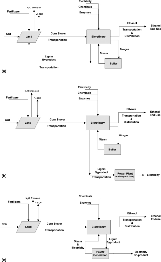
Figure 1. System boundary for ethanol production scenarios with; (a) land application of lignin byproduct (HLFB); (b) coal substitution with HLFB; and (c) onsite power generation with HLFB.
Download figure:
Standard image High-resolution imageFor the environmental performance of the biorefinery, we estimate life cycle global warming potential (GWP) for the GHGs CO2, CH4, and N2O according to IPCC 2007 for a 100 year time horizon [43]. Processes and steps are modeled in the chemical engineering software Aspen Plus 7.1 [44] and life cycle assessment SimaPro7.3.2 Software [45]. Change in soil carbon and N2O emissions from feedstock production following the application of the HLFB (for scenario 1); and residue removal and nutrient replacement (for scenarios 2 and 3) were modeled with the terrestrial ecosystem model DayCent [46] for the three counties in Iowa (Boone Co.), Maryland (Queen Anne's Co), and North Carolina (Lenoir Co.) and are discussed in Adler et al [47].
2.2. Life cycle model construction
Common inputs across the life cycle of ethanol fuel for the three scenarios include (1) production and collection of feedstock (modified for specific equipment differences in harvesting corn stover, wheat and barley straw); (2) feedstock transport from the farm to the biorefinery; and (3) the bioconversion steps pretreatment and conditioning of feedstock, enzymatic hydrolysis and fermentation. Thermal and electrical energy supply to the biorefinery and HLFB utilization are unique for each scenario. In the first scenario biogas from anaerobic digestion is used for steam generation, electricity is purchased and delivered to the biorefinery, and the byproduct is transported to land. The second scenario utilizes the same thermal and electrical energy supply as scenario one, but additionally uses a rotary dryer to dry the separated HLFB for sale to coal co-firing electric power plants; we include transportation steps to deliver the dried HLFB to the power plant. In the third scenario steam and electricity are produced onsite by integrating a boiler that takes the HLFB feed and produces electricity as a co-product. The cradle-to-gate inputs to the biorefinery, including chemicals and enzymes are inventoried based on retrofitting a biorefinery LCA model developed in [22, 48] for dilute acid pretreatment in combination with simultaneous saccharification and co-fermentation (SSCF). However, other pretreatment technologies such as autohydrolysis or steam explosion could also be considered [49, 50]. In addition to these unit operations, the process involves feedstock handling and storage, product purification, wastewater treatment, enzyme production, byproduct dewatering, product and co-product storage, and other utilities. Electricity inputs were specified based on regional electricity mixes for each site. System expansion rules were used to estimate GHG credits.
We assume harvest and collection of 50% of corn stover and 75% of wheat and barley straw within a 50 mile radius of the biorefinery to supply hourly dry biomass feeds of 83 334 kg, producing 21 808 kg per hour of ethanol. We examined a reconfiguration of the corn stover-to-ethanol biorefinery design by Humbird et al [10] with a modified biogas boiler and byproduct handling. The HLFB land amendment and coal substitution scenarios we develop assume that one fraction of the boiler feed (biogas) in the Aspen Plus model design by Humbird et al [10] is sent to a new boiler to be combusted. The dewatered HLFB (45% moisture) containing lignin and sludge from wastewater treatment is returned to lands within a 50 mile radius of the biorefinery and then land applied using liquid fertilizer spreading equipment; or dried to 20% moisture and delivered to the nearest coal power plant for direct substitution and co-firing with coal to produce electricity. Selling the HLFB as a substitute for coal in co-fired power plants would provide a co-product credit for a high carbon-intensity power source and would eliminate the uncertainty associated with assuming average electricity credits if electricity were sold as a co-product as in scenario 3. Full details on the life cycle and cost models, data, and assumptions are provided in the supporting information (SI, available at stacks.iop.org/ERL/8/025021/mmedia).
Sensitivity and uncertainty analysis was performed for model parameters judged to be significant on life cycle GHG emissions. The uncertainty analysis was undertaken using SimaPro [51] stochastic functions and Crystal Ball software. The reference case in each scenario is based on feedstock characteristics and fuel conversion measurements from Humbird et al [10] for corn stover and Aspen Plus model results. Parameter settings for the reference and stochastic analysis cases are summarized in the SI.
2.3. Site selection and biorefinery costs
The three options for producing ethanol were contrasted in three distinct US growing regions, the Midwest (Iowa), the Midatlantic (Maryland), and Southeast (North Carolina), to evaluate the effect of location on the nitrogen and carbon fluxes from the soil and its effect on the overall performance of the biorefinery. The locations chosen represent the supply area within a 50 mile radius of the biorefinery. The sites were selected based on the adequacy of the counties to supply residues at 2000 dry tons per day; the purchasing price of electricity to minimize operating cost, and the climate of the region which will affect crop residue yield, soil carbon uptake, and nitrous oxide emissions [52, 53]; see SI (available at stacks.iop.org/ERL/8/025021/mmedia) for details.
For total project investment, we assumed installed equipment costs reported by Humbird et al [10] for the same scale of facility, but modified the thermal and electrical energy equipment and costs to represent HLFB co-product use for the three scenarios (see SI). All operating costs are calculated in $2007 US for comparing with costs from literature. Ethanol production costs are calculated by dividing the total annual costs of each system by the quantity of ethanol produced. The total annual costs consist of annual capital requirements, operation and maintenance (including maintenance, consumables, labor, waste handling) and biomass feedstock (see SI for assumptions and data). We also compared the three HLFB treatment scenarios with an earlier NREL biorefinery design [9], in which the process of ethanol conversion is slightly different from the NREL 2011 [10] design and the HLFB has different nutrient characteristics. Details of the analysis results and comparison of the three scenarios of the two designs is described in the SI.
3. Results and discussion
3.1. Life cycle greenhouse gas emissions
Life cycle GHG emissions were examined using base case conditions (table 1) with average N2O emissions and change in SOC over the 20 year biorefinery lifetime and nth plant biorefinery performance; and under uncertain conditions (figure 2(c)) whereby the life cycle GHG emissions were subject to the most uncertain parameters in the model, soil N2O and change in SOC (figure 2(a)) and electricity grid variability (figure 2(b)). Life cycle GHG emissions varied by HLFB application and across sites examined (table 1, figure 2(c)). However, the HLFB land amendment scenario had the lowest mean and median life cycle GHG emissions for each location studied, coal substitution had the second lowest life cycle GHG emissions, and onsite power had the highest life cycle GHG emissions among the HLFB options. In North Carolina the coal substitution scenario had low, though positive GHG emissions under base case conditions, though under uncertainty median GHG emissions were negative and highly variable over the 95% confidence interval due to highly variable change in SOC (figure 2(b)) and also uncertain GHG emissions credits from the displaced coal. Overall, coal substitution in North Carolina had higher life cycle GHG emissions as compared to the HLFB amendment due to the soil organic carbon (SOC) credit at the Lenoir Co. site in North Carolina, which added CO2 credits to compensate for complete SOC replacement and additional storage. Although in both the HLFB land amendment and coal substitution scenarios for all sites and with consideration of uncertainty, additional GHGs were emitted due to the purchase of electricity, life cycle GHGs were lower because of mitigating the loss of SOC. In the case of the HLFB amendment no additional fertilizer application was needed due to nutrients entrained in the HLFB, which further lowered life cycle GHG emissions. In Iowa baseline direct and indirect nitrous oxide emissions for the HLFB amendment case were slightly lower relative to the coal substitute and onsite power cases, which both required synthetic N fertilizer application leading to higher relative N2O emissions, albeit considering the variability in N2O emissions with the HLFB (figure 2(a)), differences among the three uses of the HLFB are not deemed significant. Direct and indirect N2O emissions were not significantly lower among the three HLFB options in both Maryland and North Carolina, with the land amendment case being slightly lower than both coal substitution and onsite power generation in North Carolina.
Table 1. GHG emissions of life cycle components: Feedstock production, Feedstock transport, and Fuel conversion for the studied scenarios and locations. All values expressed in g CO2e/MJ of ethanol.
| Life cycle components | Boone County, IA | Queen Anne County, MD | Lenoir County, NC | ||||||
|---|---|---|---|---|---|---|---|---|---|
| Land amendment | Coal substitute | Onsite power production | Land amendment | Coal substitute | Onsite power production | Land amendment | Coal substitute | Onsite power production | |
| Feedstock production: | |||||||||
| Harvest | 12.8 | 12.8 | 12.8 | 12.8 | 12.8 | 12.8 | 12.8 | 12.8 | 12.8 |
| Nutrient replacementa,b | 0 | 5 | 5 | 0 | 5 | 5 | 0 | 5 | 5 |
| Total soil N2O emission | 3.4 | 6.9 | 6.9 | 2.5 | 3.8 | 3.8 | 2.2 | 3.3 | 3.3 |
| Change in soil carbon | 0.48 | 25.2 | 25.2 | −1.05 | 22.1 | 22.1 | −4.7 | 17.2 | 17.2 |
| Biogenic carbonb | −233.6 | −233.6 | −233.6 | −233.6 | −233.6 | −233.6 | −233.6 | −233.6 | −233.6 |
| Feedstock transport | 2 | 2 | 2 | 2 | 2 | 2 | 2 | 2 | 2 |
| Fuel conversion: | |||||||||
| Pretreatment chemicals, nutrients, enzymes | 5.9 | 5.9 | 5.9 | 5.9 | 5.9 | 5.9 | 5.9 | 5.9 | 5.9 |
| Fermentative CO2 | 45 | 45 | 45 | 45 | 45 | 45 | 45 | 45 | 45 |
| Boilerc,d | 40 | 40 | 122 | 40 | 40 | 122 | 40 | 40 | 122 |
| Transportation of HLFB | 1 | 0.6 | N/Ae | 1 | 0.6 | N/A | 1 | 0.6 | N/A |
| Electricity | |||||||||
| Process | 49.7 | 49.7 | N/A | 35.7 | 35.7 | N/A | 33.5 | 33.5 | N/A |
| Co-product | N/A | −82f | −22.3g | N/A | −82 | −16 | N/A | −82 | −15 |
| HLFB combustion | N/A | 82 | N/A | N/A | 82 | N/A | N/A | 82 | N/A |
| Fuel transport & distribution | 1 | 1 | 1 | 1 | 1 | 1 | 1 | 1 | 1 |
| Ethanol combustion | 71 | 71 | 71 | 71 | 71 | 71 | 71 | 71 | 71 |
| Net | −2.3 | 32 | 40.5 | −18.7 | 11.8 | 40.6 | −24.9 | 4.2 | 36.2 |
aIt is assumed that HLFB includes all the nutrient thus no emission from the addition of synthetic fertilizer for nutrient replacement is assumed in the land amendment scenario. bCarbon entering the biorefinery as the feedstock input. cBiogenic carbon. dBoiler emission in land amendment and coal substitute scenarios includes combusting anaerobic digestion biogas to provide steam requirements of the biorefinery while boiler emission for onsite power production includes emissions from combusting anaerobic digestion biogas and HLFB to provide steam and electricity for the biorefinery. eNot applicable. fCoal substitute scenario gains credit from offsetting coal combustion for electricity generation. gOnsite power production scenario gains credit for producing electricity and selling it to the regional electricity grid.

Figure 2. Stochastic greenhouse gas emissions (95% confidence interval and interquartile ranges) for: (a) change in soil organic carbon (SOC) and direct and indirect N2O emission for HLFB and fertilizer application at 3 studied sites, Boone, Queen Anne's and Lenoir counties; (b) electricity supply emissions for the land amendment and coal substitution scenarios for each reliability regions MRO, RFC and SERC corresponding to Iowa, Maryland, and North Carolina; the onsite power generation case supplies its own electricity; (c) life cycle emission for 3 sites and 3 scenarios of land amendment, coal substitute and onsite power production. All GWP estimates in g CO2e/MJ ethanol.
Download figure:
Standard image High-resolution imageAt the biorefinery (table 1, fuel conversion), although the HLFB amendment and coal substitution cases both have GHG emissions due to the purchased electricity and transporting the HLFB, while the onsite power generation case has a credit from the sale of surplus electricity to the regional electricity grid, boiler emissions, which use HLFB and biogas generated at the biorefinery to produce steam are higher for the onsite power case. As a result, total GHG emissions from the biorefinery, including credits are highest for the onsite power scenario in all three locations. For the coal substitution scenario, on a life cycle basis GHG emissions were lower than for onsite power generation because of directly substituting the co-product with a highly carbon-intensive power source (coal) rather than a power source composed of a grid-mixture of high and low GHG sources (coal, natural gas, nuclear, and hydro-electric).
3.1.1. GHG emission tradeoffs for biorefinery thermal and electrical energy needs.
The HLFB land application and coal substitution scenarios make use of anaerobic digestion biogas produced from the wastewater treatment section of the biorefinery. The biogas boiler simulated in Aspen Plus is sized to be much smaller than the boiler needed for onsite power generation because it is sized only for steam production as a result of purchasing electricity and selling the lignin fraction of the feedstock. Because the biogas can supply the biorefinery's steam needs, the boiler (table 1) emits less than half of the biogenic carbon in the feedstock, while storing the remaining in the HLFB that is used to replace soil carbon loss due to residue removal for the land amendment scenario; and to displace fossil CO2 emissions from the coal substitution scenario. Neither the additional transportation steps for moving the HLFB to market (to agricultural soils or to nearby coal power plants) nor the loss of the electricity co-product credit significantly affected the overall GHG balance (figure 2(c)) for the land amendment and coal substitution cases, suggesting that on a life cycle basis, alternatives to onsite power may be more beneficial. Moreover, the land application scenario points to the further GHG emission reduction benefits of non-energy use of lignin in lignocellulosic feedstocks.
The alternative to using the lignin fraction of the biomass feedstock within the biorefinery requires additional transportation of the HLFB either back to agricultural land or to a coal power plant. The lignin is separated from the cellulose and hemicellulose fractions of the feedstock following pretreatment, and in spite of the dewatering step that produces the HLFB product that resembles filter cake from wastewater treatment, the HLFB contains 45% moisture, which has a GHG and cost penalty due to shipping additional water (moisture) back to land. By contrast, the feedstock contains between 15% and 20% moisture. In spite of the moisture content, the HLFB is concentrated in lignin, containing about three times more lignin as compared to each metric ton of residue removed from the land. Assuming that fertilizer transportation trucks are used to return the HLFB to the agricultural lands 50 miles from the biorefinery, results in 1 g CO2e/MJ ethanol for the transportation of the byproduct to land.
For the coal substitution scenario we assume use of drying equipment to reduce moisture in the HLFB from 45% to 20%, prior to shipping to the nearby coal power plant. While the drying steps add capital equipment cost and energy and GHG emissions, drying is necessary for coal co-firing and it reduces transportation costs and GHG emissions.
3.1.2. Biogeochemical C and N tradeoffs of residue removal for bioenergy.
If agricultural residues are removed for bioenergy purposes there can be adverse ecological and economic impacts due to possible crop yield decline [39]. In both the coal substitution and onsite power generation scenarios, the GHG benefits of electricity co-production come potentially at the expense of soil organic carbon loss. We examined the average changes to SOC over 20 years for 50% corn stover and 75% wheat/barley straw with nutrient replacement only (for electricity co-product scenarios) and HLFB land amendment using DayCent (table 1, SOC change and N2O emissions). Agricultural soils amended with the HLFB in each location experienced smaller losses of SOC over the 20 year average (table 1) and while considering inter-annual variability in change in SOC (figure 2(a)) compared to using the 'lost' soil carbon to supply electricity to the market and displace power from fossil energy sources.
DayCent modeling results show that the carbon content of the HLFB returned to the land can compensate for the carbon that was removed with residue collection to produce biofuels. Averaged over a 20 year cycle of corn stover (table 1), wheat and barley straw removal to supply year-round feedstock, we estimate a soil carbon loss of 25, 22, and 17 g CO2e/MJ of ethanol for the scenarios that utilize the byproduct for energy in Iowa, Maryland, and North Carolina. However, HLFB amendment incurs a small SOC loss in Iowa (under 1 g CO2e/MJ), a modest gain in Maryland compared to if no amendment were returned (1 g CO2e/MJ), and a gain in North Carolina (5 g CO2e/MJ). While stochastic results that consider inter-annual variability in SOC (figure 2(a)) show a large range of change in SOC, DayCent simulations over a 20 year period show a consistent accumulation of SOC (i.e., negative GHG emissions) that tend towards mitigating SOC loss, and are thus characterized best through the 20 year average in table 1. This finding indicates that while the biomass residue can be used for ethanol production the process byproduct could be sent back to minimize the net carbon emission from the soil.
The HLFB potentially replaces N and other soil nutrients since the non-cellulosic/hemicellulosic components of the biomass are returned to the field. The HLFB (3.4% by mass, dry basis) contains additional N on top of what was in the feedstock entering the biorefinery from the ammonia used for pH conditioning that exits the biorefinery with the HLFB product. Phosphorous and potassium are also concentrated in the HLFB since almost all of the ash content gets concentrated in the HLFB stream leaving the biorefinery. We assume that all the HLFB is returned to the same land from which the biomass residue was taken. Simulation results with nutrient application (coal co-firing and onsite power scenarios) averaged over 20 years show direct and indirect N2O emission of 6.9, 3.8 and 3.3 g CO2e/MJ of ethanol for Boone, Queen Anne's and Lenoir counties, respectively, while these emissions decline somewhat to 3.4, 2.5 and 2.2 g CO2e/MJ when HLFB is applied. Therefore land application of HLFB can potentially offset or minimize using fertilizers and consequently the emissions from producing and applying them to the land. Results show that land application of the HLFB can provide carbon sequestration in all the selected sites but the level of carbon storage can differ by location.
Using the HLFB for power generation results in a credit for surplus electricity produced as a byproduct and sold to the grid, which itself has a high resulting emission. However, co-product crediting of this surplus electricity is controversial due to uncertainties in whether each average hourly electricity unit on the grid actually gets displaced by the biorefinery's co-product. To further investigate this uncertainty, we considered two extreme cases, one with perfect substitution of electricity composed of each region's average fuel mix (the most uncertain extreme, reflected in figure 2(c)) and one with no electricity credit (conservative/low risk case with zero substitution, SI table S5, available at stacks.iop.org/ERL/8/025021/mmedia). We conclude that without the co-product credit (SI table S5), and considering other uncertainties in the status of the technology as well as loss of soil carbon and N2O emissions, the lignocellulosic ethanol would not meet EISA [54] requirements of a 60% GHG reduction relative to the 2005 gasoline baseline (93 g CO2e/MJ). In contrast producing the lignin–land amendment appears to be a more sustainable means of biofuel production as opposed to utilizing it for energy recovery because the amendment stores carbon, adds nutrients, and potentially provides other soil ecosystem services.
3.1.3. Co-firing of byproduct with coal.
The option of utilizing the HLFB as a substitute for coal is an economically attractive option as it does not require a large incremental investment and the dried HLFB can be implemented immediately in nearly all coal-fired power plants in a relatively short period of time according to Basu et al [55]. There are around 40 co-firing installations in the US, about one hundred in Europe and some in other parts of the world. The majority of biomass co-firing installations use a biomass to coal co-firing ratio of about 10% on a heat input basis [55–57]. Thus we assume that 10% of the coal feed to a coal-fired power plant can be replaced with the HLFB. Greenhouse gas emissions from coal power depend on the type of coal and efficiency of the power plant. Venkatesh et al [58] demonstrate significant uncertainty in the life cycle carbon intensity of coal electricity emissions (89–106 g CO2e/MJ over a 90% confidence interval). If the HLFB is used as a substitute for coal power the electricity produced from combustion of the lignin byproduct can directly displace the electricity from coal in the grid. Results show that 82 g CO2e/MJ of ethanol avoided emission due to co-firing of the byproduct with coal (see detailed analysis in SI available at stacks.iop.org/ERL/8/025021/mmedia).
3.2. Economic analysis
Analysis of capital, operating, and total annual amortized costs for the Iowa site (table 2) shows that providing power (steam and electricity) onsite using the HLFB fed boiler (239 000 kg steam h−1), [10] adds $65.8 M to the capital cost, resulting in $121.4 million to the project. Alternatively, land applying or coal substituting the HLFB requires a small boiler to produce 103 000 kg h−1 of steam, which can be outfit with biogas produced from anaerobic digestion. The biogas fed boiler fulfils the biorefinery's steam needs for $7 million. Installation of a rotary dryer used for drying the byproduct before its transportation to the coal plant introduces an additional $4 million to the capital cost in the coal substitute scenario whereas considering onsite storage for the HLFB adds an additional $36 million to the land amendment scenario. Considering the same amount of feedstock, same ethanol production technology and ethanol production rate, the total fixed installed cost of the biorefinery for the HLFB land amendment, coal substitution, and onsite power production scenarios are $383 million, $313.5 million and $401 million, respectively. Although additional equipment is needed for the coal substitution scenario, such as a tubular dryer to reduce the moisture of the HLFB to 20%, the cost reduction of outfitting the biorefinery with a small boiler overcomes any other added fixed charges. Fixed installed cost also affects the additional costs in project capital investment (see SI).
Table 2. Cost summary comparison of scenarios of three different application of the lignin byproduct. (Note: all costs are in year 2007 US dollars.)
| Cost category | Land amendment | Coal substitute | Onsite power production |
|---|---|---|---|
| Capital costs ($/yr) | |||
| Boiler | $7 000 000 | $7 000 000 | $66 000 000 |
| Rotary dryer | N/Aa | $3 800 000 | N/A |
| Total installed equipment cost | $307 000 000 | $313 500 000 | $401 000 000 |
| Total project investment | $324 500 000 | $331 000 000 | $423 000 000 |
| Operating costs ($/yr) | |||
| Electricity purchase | $12 900 000 | $12 900 000 | −$6 200 000 |
| Byproduct transportation | $1 400 000 | $400 000 | N/A |
| Credit from selling HLFBb | −$10 800 000 | −$4 900 000 | N/A |
| Total operating cost | $103 200 000 | $108 600 000 | $97 300 000 |
| Amortized capital costc | $18 800 00 | $19 000 000 | $24 500 000 |
| Total annual cost ($/yr) | $122 000 000 | $127 800 000 | $121 400 000 |
aNot applicable. bHLFB sold for soil nutrients in land amendment scenario and as a dried coal substitute to coal-fired power plants. HLFB is not sold in onsite power production scenario. cAnnual payment of loan with 40% equity of [10].
Using a biogas boiler and purchased electricity results in a total estimated capital cost of $324.5 million and $331 million for producing ethanol with lignin byproduct for land amendment or coal substitute, respectively. This is a significant cost reduction relative to using the lignin for energy recovery with a standard Rankine cycle with a total project capital investment of $423 million. Capital cost reduction directly changes depreciation costs, which are $3.2 million and $2.9 million lower for HLFB land amendment and coal substitution, respectively.
Changes to the operating costs among the three scenarios result from many more factors than change to capital cost. Both options of land amendment and coal substitution result in adding new operating costs and reducing select other operating costs. Operating costs that are eliminated or reduced include costs of some raw materials needed for the lignin boiler and turbo-generator, income costs (e.g., sale of the HLFB), and depreciation costs since maintenance, raw material costs, labor, capital depreciation, and loan repayment costs are all lower with the small boiler without a turbo-generator.
Operating cost differences for the land amendment and coal substitution scenarios are mainly due to electricity purchase from the grid and transportation of the byproduct to land or to the coal power plant. The overall added annual operating cost for the land amendment and coal substitution scenario compared to the onsite power production scenario are $5.9 million and $11.3 million, respectively. The main difference between the two is that the land amendment scenario has higher income due to our price estimation of the HLFB owing to its nutrient (N, P, K) composition, compared to the dried HLFB substitution for coal. Another source of difference in operating costs for the two scenarios is due to transportation (mode, distance, and moisture content of the HLFB) in delivering the HLFB to its end use. Transportation and amendment of the HLFB to land adds approximately $1.4 million per year for this option. The land amended HLFB has a moisture content of 45%, whereas the coal substitute's moisture content is 20%. The total annualized cost, including the amortized capital cost assuming 40% equity is $122 million for land amendment, $127.8 million for coal substitution, and $121.4 million for onsite power production. The main difference in total annualized costs among the three scenarios centers around the cost of equipment to provide steam and/or electricity, operating costs due to purchasing electricity (land amendment and coal substitution scenarios), and value of the resulting HLFB produced for generated income for the biorefinery.
3.2.1. Allocating price for selling the lignin byproduct.
During biofuel conversion most of the nutrients from the biomass plus additional nutrients added during conversion partition into the HLFB, thus using the HLFB as a soil amendment returns most of those nutrients to the soils. We therefore assume the HLFB supplies the soil with nutrients removed with residue removal, and estimate a price for the HLFB based on the market price of nutrients concentrated in the HLFB. We assume a price of $50/dry ton of HLFB based on its nutrient values relative to the price of the fertilizers [59] independent of the location. This price does not include the value of SOC replacement, which is factored into the land amendment life cycle GHG emissions scenario, but not in the coal substitution or onsite power. We consider scenarios that reflect a market value for SOC in section 3.3.
3.2.2. Byproduct for electricity generation.
To be competitive with coal, biomass should be priced 20% below the price of coal to offset the cost of equipment retrofits [60]. We assume that equipment retrofitting is not needed with the HLFB feedstock since it has undergone size reduction at the biorefinery. We priced the HLFB based on its energy value relative to the 2009 price of coal in the three states [61]. Reducing the moisture of the HLFB from 45% to 20% is necessary for reducing transportation costs and increasing the material's energy density (the LHV increases from 9.8 to 14.7 MJ kg−1). The dried HLFB proposed for the coal substitution scenario has a higher heating value compared to wood and a lower selling price according to cost analysis (table 3). The price that electric utilities pay for coal varies by state and depends on the type of coal, demand and the proximity of coal mines which affects the transportation cost of the coal. Prices of coal to be used in electric utility plants in the corn-belt states range from $17 to $60 per ton while in other states it can go up to $230 per ton (e.g., in the Midatlantic). As a reference point, operating costs reflected in table 2 for Iowa consider coal priced at $25/metric ton and the HLFB priced at $18.8/metric ton. The biorefinery in Iowa profits from selling the byproduct (31 metric tons h−1) to industry, which reduces the operating cost to 128 million dollars for the HLFB containing 20% moisture. Cost of the transportation in this option will be around $400 000 per year which can be done by truck to send the HLFB to coal plant within 50 miles of the biorefinery. We present results of the economic analysis of the ethanol production scenarios for other states in the SI (available at stacks.iop.org/ERL/8/025021/mmedia). According to the results, economics of the biorefinery changes based on the type and the price of the coal available in each region as the energy content of the coal (MJ kg−1) and its price directly affect setting the price ($/MJ) for HLFB. These analyses suggest the Southeast US region as a potential area for co-firing option with lower operating cost.
Table 3. Prices of feedstocks for biofuel or electricity production.
| HLFB (high moisture) | HLFB (low moisture) | Wooda | Coal | |
|---|---|---|---|---|
| Moisture (wt%) | 45 | 20 | 20.0 | 7.6 |
| HHV (MJ kg−1) | 10.5 | 15.8 | 14.6 | 21b |
| Price ($/dry t delivered) | 12.5c | 18.8c | 25.9 | 25d |
aData are taken from Basu et al [55]. bKim and Dale [62]. cMaximum delivery cost for byproduct in order to be competitive with wood feedstock at the cost of $25 for coal. dEIA [63].
3.3. GHG abatement costs and sensitivity of operating costs and HLFB selling price
We combine results from the life cycle GHG emissions and techno-economic analysis to compare the GHG abatement costs for each scenario relative to replacing gasoline (figure 3). We evaluate two cost cases for the land amendment scenario. The first case, which we designate as high (H), applies the same feedstock harvest price as the coal substitution scenario. The second case, which we designate as low (L), considers a $20/dry metric ton reduction in feedstock harvesting cost resulting from economy of scale effects at higher corn stover harvesting rates discussed by Graham et al [64] that could occur due to SOC replacement. We evaluate the effect of pricing soil organic carbon (SOC) replacement through applying a market value ranging from $20, $50, and $100/metric ton CO2 to the HLFB on abatement cost (figure 3(a)); and the effect of a universal (life cycle) carbon tax at $20, $50, and $100/metric ton of CO2e for ethanol and gasoline (figure 3(b)). To be conservative, we use life cycle GHG emissions set to the 75th percentile of the 95% confidence interval of results (figure 2(c)), and note that the onsite power case without electricity crediting (i.e., the most uncertain extreme) is not considered here due to not meeting RFS2 [65] requirements for cellulosic biofuels.

Figure 3. GHG abatement cost and site-specific biorefinery operating cost for the HLFB land amendment, co-firing and onsite power production scenarios to substitute gasoline for the three selected sites with (a) soil carbon valuation; and (b) a universal carbon tax. Both scenarios consider high (H) and low (L) feedstock harvesting prices for HLFB land amendment due to lower feedstock harvest costs at increasing removal volumes when soil carbon is replaced. Each ethanol production scenario is compared to the 2007 production price of gasoline with life cycle GHG intensity 93 g CO2e/MJ from [53].
Download figure:
Standard image High-resolution image
For each scenario in figure 3 we summarize the state-specific operating costs for producing each unit of ethanol (per MJ basis), which takes into account electricity price variation by state, its effect on HLFB selling price, and how that affects operating costs. The price of electricity that is either sold (onsite power) or purchased (land amendment and coal substitution) by region impacts the operating cost. For Queen Anne's County this dynamic results in the highest operating costs among other counties when electricity is purchased (land amendment and co-firing options) and the lowest operating cost where electricity is sold (onsite power production).
Results with SOC valuation (figure 3(a)) indicate that abatement costs are lower for onsite power and coal substitution when feedstock harvest prices are the same for all scenarios (the high case for land application) and no SOC valuation, except for Boone Co., IA, which is roughly on par with onsite power generation. However, location is significant among the HLFB-energy scenarios, with Lenoir Co. having the lowest abatement cost for coal substitution. This point highlights the location dependency on economic and GHG tradeoffs due to location-specific biogeochemistry and state electricity prices. When we place a value on SOC, the abatement costs for land amendment decline significantly even for the high feedstock price, and at a SOC value of $100/ton CO2, land amendment becomes more attractive in Lenoir Co. At low harvest costs for land amendment with SOC valuation, land amendment is on par with onsite power generation for Queen Anne's Co., and it represents the most attractive abatement option for the other two counties.
When there is a universal carbon tax across all markets, there is much less variability among the GHG abatement costs across the scenarios compared (figure 3(b)). When there is no carbon tax, the land amendment-low (L) feedstock harvest case has the lowest abatement cost among all options (except in the case of Queen Anne's Co., which is on par with onsite power generation), but coal substitution has the lowest abatement cost if high feedstock prices entail for the land amendment option. Adding a carbon tax across the life cycle of both the ethanol and gasoline reduces the influence of SOC replenishment due to valuing carbon evenly across the life cycle, particularly for displacing coal power. Applying a higher tax of $50 and $100/ton of CO2 makes all the values of abatement cost negative making the co-firing option in Lenoir Co. the most favorable and least costly option (if harvest prices are high for land amendment). Abatement cost in Boone Co. is low for land amendment but not significantly different from onsite power with high feedstock harvest prices among all the counties. Low abatement cost for land amendment in Boone Co. results from low electricity prices and a negative life cycle carbon emission for this location. Land application in Queen Anne's Co. has the highest cost and coal substitution second highest due to the higher incremental cost of electricity among sites, suggesting that onsite power production could be the more cost effective option in the Midatlantic region.
4. Conclusion
There is much opportunity to develop alternatives to producing electricity from the lignin portion of biomass used to produce alcohol from the cellulose and hemicellulose fractions. Our main objective in this paper explored the cost and GHG tradeoffs of providing long-lived soil carbon to agricultural soils from the portion of agricultural residues that remains in the soil if the residues were not collected for biofuel production. If soil carbon replacement can allow for higher residue removal from land just to the point of avoiding erosion, and thus reduce feedstock harvesting cost according to Graham et al [64], the economics of residue removal amount to negative GHG abatement costs for biorefineries designed to produce a land amendment rather than energy co-products. Although there is expected variability in the level of SOC replacement with the carbon-rich amendment as evidenced by variability among DayCent results for the sites we investigated, most sites considered in this work lost little SOC relative to not removing residue at all. On a life cycle basis returning lignin to land after extracting the fermentable sugars from the residue results in greater avoided GHGs than if no residue were removed. This finding is significant for techno-economic analysis of potential future second generation biorefinery design. In particular, if economy of scale residue harvest prices coincide with minimizing SOC loss, the costs would work out favorably for returning a not only nutrient-rich biorefinery byproduct to the land, but also one with much soil carbon value.
Acknowledgment
The authors greatly thank two independent referees who provided valuable comments on this manuscript.