
Abstract
Projections of future changes in weather extremes on the regional and local scale depend on a realistic representation of trends in extremes in regional climate models (RCMs). We have tested this assumption for moderate high temperature extremes (the annual maximum of the daily maximum 2 m temperature, Tann.max). Linear trends in Tann.max from historical runs of 14 RCMs driven by atmospheric reanalysis data are compared with trends in gridded station data. The ensemble of RCMs significantly underestimates the observed trends over most of the north-western European land surface. Individual models do not fare much better, with even the best performing models underestimating observed trends over large areas. We argue that the inability of RCMs to reproduce observed trends is probably not due to errors in large-scale circulation. There is also no significant correlation between the RCM Tann.max trends and trends in radiation or Bowen ratio. We conclude that care should be taken when using RCM data for adaptation decisions.
Export citation and abstract BibTeX RIS

Content from this work may be used under the terms of the Creative Commons Attribution-NonCommercial-ShareAlike 3.0 licence. Any further distribution of this work must maintain attribution to the author(s) and the title of the work, journal citation and DOI.
1. Introduction
Projections of future climate can be used by policy makers and planners to inform adaptation choices. The occurrence of weather extremes is of particular interest in this respect, as their impact on society is large. Numerous studies have shown that their nature, scale and frequency is changing and will change further due to climate change (IPCC 2012). In particular, heat waves and high temperatures are shown to increase significantly in frequency and severity in a large number of regions in the world (Clark et al 2006, Fischer and Schär 2010). Observations indicate that the land surface temperature in north-western Europe is increasing at least twice as fast as the global average (van Oldenborgh et al 2009), which is not reproduced by models. Models do indicate that temperature extremes tend to increase faster than the mean temperature (Clark et al 2006, Sterl et al 2008).
The main tools to generate projections of climate are global circulation models (GCMs). The relatively coarse spatial resolution of such models (>100 km) makes them of limited use for local planning and adaptation decisions. To provide information on the finer spatial scales, regional climate models (RCMs) are employed. These are atmospheric models that run on a limited geographical area, taking boundary conditions from a GCM. Their finer spatial resolution allows for the incorporation of more local details such as orography and land use, and representation of smaller scale dynamical processes such as some aspects of land-surface interactions. However, Christensen et al (2008), Buser et al (2009) and Boberg and Christensen (2012) report large biases in RCM temperatures over Europe. Although bias corrections are often applied, Maraun (2012) shows that this may hardly improve projections for summer temperature in large parts of Europe, mainly due to time dependence in the biases. Moreover, Lorenz and Jacob (2010) find that RCMs underestimate trends in annual and seasonal averaged temperatures. Nonetheless, RCM trends in heat extremes are used in several studies to formulate expectations for the future (e.g. Barriopedro et al (2011) and Frías et al (2012)).
In this letter we study trends in the hottest day of the year Tann.max, i.e. the annual maximum of the daily maximum 2 m temperature Tmax, as produced by a large ensemble of RCMs run for the historical period 1961–2000. The RCMs take atmospheric boundary conditions and sea surface temperatures (SST) from ERA-40 (Uppala et al 2005), ensuring that all difference between their output stems from differences within the RCMs themselves. The RCMs are validated against observations and reanalyses. Because ERA-40 is used for both the boundary conditions and as part of the validation data set, discrepancies can be attributed to the RCMs themselves. We have not studied RCMs driven by GCM boundaries. Since GCMs do not aim to reproduce the current realization of our climate but only its statistical properties, direct comparison to observations is not straightforward. Using GCM boundaries further has the drawback of mixing up uncertainties and errors in both RCMs and GCMs.
We only study land area, since better direct observations are available here. Our region of study, to which we will refer as 'north-western Europe' (NW EU), is the area ranging from 44° to 59° N and from 10° W to 16° E.
2. Observations
As the main representation of realized climate we use the state-of-the-art daily gridded data set E-OBS version 6.0 (Haylock et al 2008). This data set contains land station data of daily maximum temperatures (Tmax) interpolated on a 0.22° (∼25 km) rotated polar grid. The interpolation of station data to grid boxes smooths the magnitude of extremes, making the data directly comparable to the area-averaged values of RCM grid boxes (Haylock et al 2008). The effect of possible over-smoothing on trends in Tann.max was explicitly studied by Hofstra et al (2010) and found to be small, in particular in areas with a high station density compared to the decorrelation scale of this variable, like NW EU.
The trends in Tann.max from E-OBS are presented in figure 1(a). Although the type of studied variable (block maxima) would suggest the use of a generalized extreme value (GEV) model for trend fitting, it was verified (see supplementary material available at stacks.iop.org/ERL/8/014011/mmedia) that Tann.max, as a moderate extreme, is not in the GEV regime. We therefore use a simple linear regression to determine the trend. The residuals of this regression were confirmed to be normally distributed with constant variance and no auto-correlation (see supplementary material available at stacks.iop.org/ERL/8/014011/mmedia). This allows standard statistical methods (t-test) to determine confidence intervals and check for statistical significance (indicated with dots in figure 1).
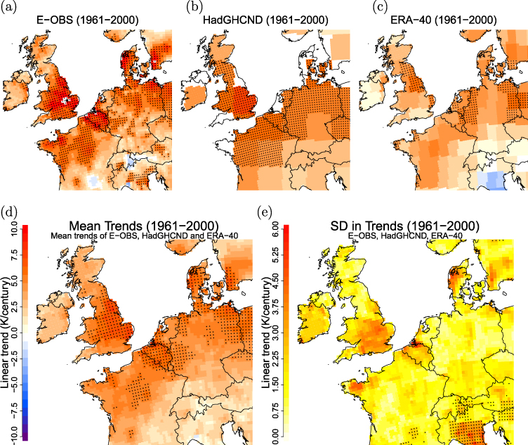
Figure 1. Linear trends in the annual maximum of the daily maximum 2 m temperature Tann.max over 1961–2000 from different (semi-)observational data sets: (a) the E-OBS data set, (b) the HadGHCND data set and (c) the ERA-40 reanalysis. The mean of these trends, interpolated on the E-OBS grid, is shown in (d). In all these maps, dots indicate significant trends. The standard deviation of the three trends is shown in (e), with dots indicating where the spread exceeds the trend in the mean.
Download figure:
Standard imageStation data are included in E-OBS with minimal demands on homogeneity. Relocation of stations, land-use change in the surrounding area, or change of instrumentation will introduce inhomogeneities in Tmax and its trend. The high trends in Belgium and the south-east of England may be influenced by such effects. To be able to estimate the error in the trends we compare E-OBS with other data sets.
The HadGHCND data set (Caesar et al 2006) is set up for daily extremes in particular and uses ground station data interpolated on a much coarser grid (3.75 × 2.5°) than E-OBS. HadGHCND is not fully independent of E-OBS, as the overlap between used stations in Europe is considerable. Although in general the trends are somewhat lower, it is no surprise that the large-scale picture is the same as that of E-OBS (figure 1(b)).
A more independent check can be provided by the ERA-40 reanalysis (Uppala et al 2005). Although 2 m temperatures from land stations are assimilated in ERA-40, the way this is done makes the atmospheric reanalysis only weakly dependent on them (Simmons et al 2010). As can be seen in figure 1(c), the ERA-40 trends compare reasonably well with both gridded data sets.
The trends in E-OBS are highest, probably in part because averaging over larger areas in the other data sets smooths out the highest trends. We checked the date of occurrence of Tann.max, and find the differences between the data sets to be less then 2 days in almost all cases.
We will consider the mean of the trend in Tann.max in the three observational data sets as the best estimate of the 'true' trend over the 1961–2000 period (figure 1(d)), and use this as our reference. The coarser data sets have been regridded onto the E-OBS rotated polar grid using nearest neighbour interpolation. To get a quantitative estimate of the uncertainty in the trends in observations, we plotted the standard deviation (σ) of the three trends in figure 1(e). Note that there are large areas where HadGHCND has no data. In these grid points, the mean and standard deviation of only the other two data sets is considered.
Over most of the area, σ < 2 K/century, except where HadGHCND has no data. A notable exception is the Po Valley, where ERA-40 finds negative trends in Tann.max and consequently, σ is larger than the trend itself. Comparing with trends in ERA-interim (Dee et al 2011) for the overlapping period (1979–2001) suggests this is mainly an artefact of ERA-40, as trends are positive in the updated reanalysis.
3. Regional climate models
The RCM integrations studied in this comparison are all taken from the ENSEMBLES project (Van der Linden et al 2009), in which a large number of different regional climate models was run for the historical period 1961–2000. Here we consider 14 of the highest resolution integrations, with an average grid distance of about 0.22° or 25 km in both longitude and latitude. Most of the models use the same rotated polar grid as E-OBS. The output from simulations run on a different (but approximately equally fine) grid are mapped onto the same grid by distance weighed averaging.
The outcomes of RCMs are subject to a number of uncertainties. The most important are varying boundary conditions, natural variability (both within the RCM and from the boundaries) and RCM formulation. For the current study we concentrated on the ensemble of ERA-40 driven RCMs, and thus boundary condition uncertainty can be ignored. As we have shown in figure 1, ERA-40 trends are consistent with observations. Therefore, the effect of the boundary conditions on differences between RCMs and observations is considered to be small. Differences between models can thus be attributed to natural variability or RCM formulation.
Since only a single ensemble member of each RCM was available, we estimate natural variability by considering the variability of the time series. For this we first calculate the residuals, i.e. the difference between the actual value of Tann.max and the fitted trend line. Confidence intervals are then calculated by comparing the variance of the residuals to quantiles of the t distribution (von Storch and Zwiers 1999) under the assumption that the residuals of Tann.max show no year-to-year correlation. We checked this to be true for the studied area (see supplementary material available at stacks.iop.org/ERL/8/014011/mmedia for details).
Part of the variance in the RCM output is determined by the boundary conditions and thus shared by all models. As we use boundary conditions from a reanalysis, even the observations will share most of this variance. When comparing trends in models among each other or with observations we should correct for this shared variance. We find a correlation coefficient r = 0.48 ± 0.07 between the residuals in ERA-40 and the RCMs, yielding a variance 'explained' by the boundary variability of r2 ≈ 0.25. For inter-comparisons the confidence intervals, as for example shown in figure 2, should therefore be reduced by this fraction.
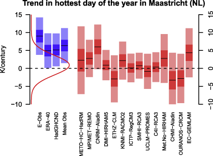
Figure 2. Trends in observations and simulations in a single grid box near Maastricht, The Netherlands (51°0' N, 5°48' E). Blue bars represent the observations, red bars represent 14 different RCMs, all with ERA-40 boundary conditions. The black lines are the best estimates for the trend in Tann.max. The darker colours show 50%, the lighter colours 95% confidence intervals due to internal variability. About a quarter of this uncertainty is due to natural variability in the boundary conditions. The red curve on the left is a normal distribution fitted around the RCM best estimate trend values.
Download figure:
Standard imageThe RCM model error is sampled by the ensemble of 14 models. By treating this as a probabilistic uncertainty, we make the implicit assumption that the used RCMs span up the space of possible, reasonable formulations of such models to a sufficient extent. Although this assumption might be too strong to be justified (see e.g. Pennell and Reichler (2011)), there is at present no better alternative.
4. Comparing observations and RCMs
We first compare the trends in E-OBS, HadGHCND and ERA-40 with the trends in the different ENSEMBLES simulations in a single grid box (51°0' N, 5°48' E, near Maastricht, the Netherlands), figure 2. The RCM ensemble clearly underestimates the observed trend. In fact, every individual RCM underestimates the trend in Tann.max with respect to the observations in this grid box. None of the RCMs find a statistically significant trend (i.e. their 95% confidence interval includes zero), whereas all observed trends are significant (p < 0.01 for E-OBS and HadGHCND, p < 0.05 for ERA-40). Nonetheless, some RCMs are clearly better in reproducing the trend than others; notably, the two highest simulated trends are close to the observed value.
There is considerable spread in RCM trends (μ = 0.9, σ = 2.7 K/century, see figure 2), as well as in trend uncertainty due to natural variability (shown by the coloured confidence intervals). On average, the variance in both Tann.max and in daily summer (JJA) temperatures (not shown) is slightly larger in the RCMs than in the observations, but again with large inter-model differences. Note that, as mentioned in section 3, about a quarter of the uncertainty around the RCM trends is due to natural variability inherited from the ERA-40 boundaries, and thus shared by all models and observations.
What is seen in figure 2 extends to large areas of NW EU. figure 3(a) shows that the median of RCM trends is low over most of NW EU, compared to figure 1(d). To quantify this further, figure 3(b) shows that in most grid points the number of RCMs for which the trend exceeds the observations is very small. Only in south-western Europe, where observed trends are relatively low, we find areas where equal numbers of RCMs under- and overestimate the trend. This extends the findings of van Oldenborgh et al (2009), who show a similar underestimation of trends by GCMs in NW EU.
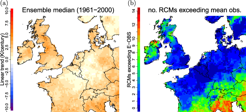
Figure 3. Comparing linear trends in the annual maximum of the daily maximum 2 m temperature over the 1961–2000 interval in observations and models; RCMs driven by the ERA-40 reanalysis. (a) The ensemble median of trends from the models on the same scale as the mean observation map in figure 1. (b) The number of RCMs for which the best estimate of the trend exceeds the best estimate of the trend in the mean observations; blue colours indicate that RCM trends are smaller than observed trends.
Download figure:
Standard imageAs in the Maastricht grid box, the simulations with the highest trends in Tann.max on average only slightly underestimate observed trends, although they do not reproduce the spatial patterns seen in figure 1(d) (not shown). The least performing models produce negative trends in Tann.max over most of NW EU (not shown). The disagreement is not statistically significant for each individual RCM, leaving the possibility that it is caused by random fluctuations. However, the ensemble samples this natural variability as well as model spread, so the fact that almost all RCMs underestimate the trend makes it very unlikely that natural variability is the main cause of the discrepancy.
5. Discussion
It is clear that some important aspect of the occurrence of moderate temperature extremes is missing from the models, and we investigated some possible aspects. It is unlikely that discrepancies can be explained by errors in sea surface temperature (SST), as the RCMs take SST from ERA-40, which in turn uses HADISST and NOAA/NCEP observations (Uppala et al 2005). These observations for the North Sea should be quite reliable as this is a well-sampled region even in the pre-satellite era. Another option is that the large-scale circulation is represented poorly in the RCMs. It is prescribed at the boundaries, but the domain is large enough for the models to generate deviations in their interior in summer (Plavcova and Kysely 2011). However, studying the same RCM ensemble, Sanchez-Gomez et al (2009) found only 15–20% of days in summer had a weather regime different than ERA-40. We checked circulation patterns on 6 of the hottest days between ERA-40 and one of the RCMs that showed a trend close to the ensemble median, and found no large deviations. We therefore conclude that the large-scale circulation is not likely to be the main cause of the difference in trends.
We also considered some components of the local energy balance, although a full account of this is beyond the scope of this paper. We looked for correlations between trends in Tann.max and radiation (both long and short wave) and turbulent surface heat fluxes (sensible and latent heat) in the RCM ensemble. Direct comparisons with observations are not made, as reliable data sets for the region under consideration do not exist.
The trend in Tann.max in E-OBS may be due to an underlying trend in downward short wave radiation SW↓, either from changes in aerosol loading or trends in cloud cover on hot days. In that case we would expect RCMs with a large positive trend in SW↓ to show a larger trend in Tann.max. figure 4(a) shows a scatter plot of those trends for the grid box closest to Maastricht. To allow for a build-up of heat, we have considered SW↓ averaged over the 5 day period leading up to and including the hottest day. There is no significant relationship between the trend in Tann.max and SW↓ (p = 0.278 on a standard t-test), indicating this is not the main problem.
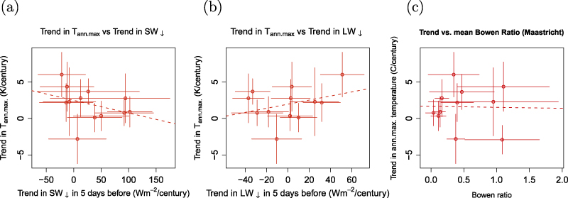
Figure 4. Scatter plots of trend in Tann.max versus (a) trend in SW↓, (b) LW↓ and (c) average Bowen ratio B in Maastricht, The Netherlands. Whiskers indicate uncertainty of the trends (1σ) due to natural variability. Dashed lines show the fitted regression line.
Download figure:
Standard imageAnother possible explanation for the trends in the observations could be an increase in trapping of long wave radiation by clouds or atmospheric water vapour and other greenhouse gases, leading to an increase in LW↓. Maraun (2012) reports a large spread in the trends in cloud cover in RCMs over NW EU, which would be consistent with the large spread in Tann.max trends found here. We would then expect RCMs that better represent this process (i.e. with a positive trend in LW↓ of the 5 days leading up to the hottest day) to show larger trends in Tann.max. figure 4(b) shows there is no significant relation (p = 0.292) and thus no strong evidence for long wave trapping to be the problem.
Soil moisture and land-atmosphere feedbacks can play a large role in local heat build-up (Fischer and Schär 2009, Jaeger and Seneviratne 2011, Mueller and Seneviratne 2012). On wet soils, part of the incoming energy is used for evaporation of water, and transported away as latent heat. When the soil dries out, more energy becomes available for heating the air (sensible heat). A good measure of this drying effect is the Bowen ratio B, the ratio of sensible over latent heat. When B > 1, the soil is dry and warm days will become hotter. If soil drying plays a key role in Tann.max trends in the real world, we would expect dryer models, with a higher average Bowen ratio, to find more realistic (i.e. higher) trends. Again, no such relation is found within the ensemble (figure 4(c)).
In conclusion, we could not identify an obvious cause of the discrepancy between RCMs and observations. The (trends in) the components of the energy balance are too noisy. A sensitivity study where the effects of different processes in RCM simulation of heat extremes are thoroughly tested could clarify this issue.
6. Conclusions
We have compared linear trends in moderate heat extremes (hottest day of the year) as modelled by Regional Climate Models over north-western Europe with observations in the period 1961–2000. A strong and significant trend is found in observations over this period. However, the ensemble median of the 14 RCM ensemble under study strongly underestimates this trend. Despite a large inter-model variability, over extended areas not a single RCM can match the trends in observation. Poor representation of large-scale circulation is ruled out as a cause for this discrepancy, and we show that there is no relation between performance of the simulations and trends in downward short wave radiation, long wave radiation or Bowen ratio in the models. More study is needed to unravel the cause of this bias in trends. Care should be taken in using RCM data for making planning and adaptation decisions.
Acknowledgments
Research underlying this paper was funded by the Netherlands Organization for Scientific Research (NWO) and Program Knowledge for Climate (Kennis voor Klimaat). We acknowledge the E-OBS data set from the EU-FP6 project ENSEMBLES and the data providers in the ECA&D project. The ENSEMBLES data used in this work was funded by the EU-FP6 Integrated Project ENSEMBLES (Contract number 505539) whose support is gratefully acknowledged. We thank Gerard van der Schrier (KNMI) and Bert Holtslag (WUR) for useful discussions on observations and Dick Dee (ECMWF) for detailed information on ERA-40. We thank the two anonymous reviewers for their comments, which have improved the paper considerably.