

Abstract
A sequence of global ocean circulation models, with horizontal mesh sizes of 0.5°, 0.25° and 0.1°, are used to estimate the long-term dispersion by ocean currents and mesoscale eddies of a slowly decaying tracer (half-life of 30 years, comparable to that of 137Cs) from the local waters off the Fukushima Dai-ichi Nuclear Power Plants. The tracer was continuously injected into the coastal waters over some weeks; its subsequent spreading and dilution in the Pacific Ocean was then simulated for 10 years. The simulations do not include any data assimilation, and thus, do not account for the actual state of the local ocean currents during the release of highly contaminated water from the damaged plants in March–April 2011. An ensemble differing in initial current distributions illustrates their importance for the tracer patterns evolving during the first months, but suggests a minor relevance for the large-scale tracer distributions after 2–3 years. By then the tracer cloud has penetrated to depths of more than 400 m, spanning the western and central North Pacific between 25°N and 55°N, leading to a rapid dilution of concentrations. The rate of dilution declines in the following years, while the main tracer patch propagates eastward across the Pacific Ocean, reaching the coastal waters of North America after about 5–6 years. Tentatively assuming a value of 10 PBq for the net 137Cs input during the first weeks after the Fukushima incident, the simulation suggests a rapid dilution of peak radioactivity values to about 10 Bq m−3 during the first two years, followed by a gradual decline to 1–2 Bq m−3 over the next 4–7 years. The total peak radioactivity levels would then still be about twice the pre-Fukushima values.
Export citation and abstract BibTeX RIS

Content from this work may be used under the terms of the Creative Commons Attribution-NonCommercial-ShareAlike 3.0 licence. Any further distribution of this work must maintain attribution to the author(s) and the title of the work, journal citation and DOI.
1. Introduction
As a consequence of the magnitude 9.0 Tōhoku earthquake and subsequent tsunami hitting the east coast of Japan on 11 March 2011 the Fukushima Nuclear Power Plants (NPPs) were severely damaged and radioactive material was released to the atmosphere as well as to the ocean (Buesseler et al 2011). Samples of sea water collected off the NPPs by the Tokyo Electric Power Company (TEPCO) and the Japanese Ministry of Technology (MEXT) in the weeks after the incident indicated extremely high levels of radioactivity, as far as 30 km offshore (Fukushima Nuclear Accident Update Log by International Atomic Energy Agency, www.iaea.org/newscenter/news). Radioisotopes discharged from the plant included both short-lived isotopes like 131I (with a half-life of 8 days) and long-lived isotopes such as 137Cs (half-life of 30 years). Some fraction of these long-lived isotopes is associated with particles (review provided by Dietze and Kriest (2011)) and accumulates in the food chain (IAEA 2004 and Schiermeier 2011), with as yet unknown consequences for marine organisms in the area (Garnier-Laplace et al 2011). A substantial part of the 137Cs input is expected to be carried away by the swift near-coastal currents (http://sirocco.omp.obs-mip.fr/outils/Symphonie/Produits/Japan/SymphoniePreviJapan.htm), and dispersed over broader regions.
Previous studies of the radioactive fallout due to the nuclear weapon tests during the 1950s–60s and the Chernobyl disaster in 1986 suggested that 137Cs behaves in seawater approximately like a 'conservative' dissolvable tracer (Buesseler et al 1990, Buesseler 1991, Buesseler et al 2011), with its distribution on decadal timescales primarily governed by physical transport processes (Bowen et al 1980, Staneva et al 1999, Tsumune et al 2003). The dispersal by ocean currents was identified as a main mechanism determining the observed distribution of the 137Cs concentrations in the surface waters of the North Pacific in the 1970s: a decade after the peak input from the weapon tests (1961/62), highest concentrations occurred in the eastern basin, off the west coast of North America, although reconstructions suggested that the fallout had been concentrated in the western basin (Folsom 1980). The characteristics of the observed-1970s 137Cs-distribution were broadly captured by ocean model simulations, confirming that a large amount of 137Cs fallout must have been advected from the western to the eastern North Pacific within a decade (Tsumune et al 2003).
From an oceanographic point of view the main difference between the 1960s' weapon tests fallout and the recent discharge of artificial radionuclides off Japan are the spatial and temporal characteristics of the input. Analyses of data indicated peak ocean discharges from the stricken power plants in early April, rapidly decreasing by a factor of 1000 during the following weeks (Buesseler et al 2011). Although a continued release of radioactivity due to polluted groundwater and river discharge contributed to enhanced concentrations in the coastal waters over several months (http://ajw.asahi.com/article/0311disaster/fukushima/AJ201111250019), as a first approximation it is assumed that a significant portion of the direct oceanic discharge occurred in terms of a short-term pulse to the near-coastal areas. The total amount of 137Cs directly discharged during the period of 12 March–30 April 2011 in the ocean was estimated to be 4 PBq (Kawamura et al 2011), with an additional deposition of similar magnitude (5 PBq) for the atmospheric fallout into a wider area of the western North Pacific during the first days after the NPPs' explosion. Other studies suggested higher atmospheric deposition values (e.g. 36.6 PBq, Stohl et al 2012), reflecting a significant uncertainty of currently estimated release rates (Chino et al 2011). Preliminary assessments of the initial oceanic spreading were provided by operational modelling efforts (http://sirocco.omp.obs-mip.fr/outils/Symphonie/Produits/Japan/SymphoniePreviJapan.htm) and hindcast simulations. The numerical simulations suggested a swift dispersal of both the direct oceanic discharge and the near-coastal atmospheric deposition by the intense fluctuating currents and tidal motions over the continental shelf, with streaks of high tracer concentrations rapidly extending beyond the shelf break. Simulations with a coupled physical–biogeochemical ocean model broadly indicated two phases in the initial dispersion: an accumulation on the shelf during the first weeks, followed by increasing outflow to the open ocean after about 1–2 months (Dietze and Kriest 2012). While the actual pathways are related to the initial ocean state, their experiments showed relatively little sensitivity of the net export to the open ocean, i.e., a rather robust net evolution in the integral characteristics of the tracer patch over the following months.
Building on these findings, a suite of global ocean circulation models with different representations of mesoscale eddies is used here, to address the question of the long-term dispersion, i.e., on timescales of years to a decade, of long-lived radionuclides in the Pacific Ocean.
2. Method
2.1. Ocean circulation model
The model simulations are based on NEMO (Madec 2008), utilizing configurations developed in the Drakkar framework (The DRAKKAR Group 2007). The model configurations mainly differ in their horizontal resolution (nominally 0.5°, 0.25° and 0.1°; the latter realized by a 'two-way nesting'-approach (Debreu et al 2008) in which a 0.1°-mesh for the North Pacific was embedded in the 0.5°-mesh for the global ocean), allowing to explore the effect of mesoscale eddy variability on the tracer dispersal: typical eddy scales in the mid-latitude (30°–40°N) North Pacific are ∼100 km (Chelton et al 2007); these scales are resolved to different degrees by the 0.25°- and 0.1°-configurations (their mesh sizes in the North Pacific are ∼22 km and ∼9 km, respectively); they are not resolved in the 0.5°-model (∼45 km) where the effect of eddies is parameterized by a GM-scheme (following Gent and McWilliams 1990), with a mixing coefficient related to the growth of baroclinic instabilities (Treguirer et al 1997) but limited to 1000 m2 s−1. All model configurations use 46 vertical levels; layer thickness increases with depth. Turbulent vertical mixing is simulated with a TKE scheme (Madec et al 1998).
The model experiments were initialized with the climatological temperature (T) and salinity (S) fields of the World Ocean Atlas (Levitus 1998). The forcing is built on the atmospheric reanalysis products ('CORE' forcing) developed by Large and Yeager (2009) covering the period 1948–2007. Since the future atmospheric conditions are unknown, the forcing to simulate the tracer distribution is based on the last 10 years of the CORE forcing.
2.2. Tracer simulation
Assuming that 137Cs essentially behaves as a 'conservative' tracer or 'dye', its spreading mainly determined by advection and diffusion processes (Bowen et al 1980, Buesseler et al 2011), the tracer simulation follows the same evolution equations as those used for T and S. The simulation thus ignores possible effects of biological processes which might lead to accumulation of 137Cs in areas of high biological productivity, and potentially affect vertical tracer distributions due to adherence to sinking particles (see discussion by Dietze and Kriest (2011)), but takes into account the radioactive decay (half-life of 30 years).
Since the basin-scale models employed here cannot adequately capture the initial dispersion process, the tracer discharge was evenly distributed over a near-coastal area, with a width corresponding to the mesh size of the 0.5°-model. The influence of the along-shelf extent of the tracer injection area was tested in a series of 10 year long sensitivity runs with a variation in the size of the release area, but found to have relatively little effect on the longer-term tracer distributions. For the main model integrations, a rather large input area was chosen consisting of (or, equivalent to) three 0.5°-grid cells along the shelf, resulting in a swath of about 150 km × 45 km off northeastern Japan; due to this size it may also account for some atmospheric deposition in the vicinity off Fukushima (Stohl et al 2012, Kawamura et al 2011). The size of the input area was kept the same for the higher-resolution models.
The tracer release in the surface layer was started in mid-March from one of the last years of the available forcing period (henceforth referred to as time 0). The choice of the year, i.e., the effect of the initial distribution of currents and eddies in the input area was examined in a set of sensitivity experiments (see section below). In order to assess the relevance of the (not precisely known) discharge history, injection pulses with constant tracer fluxes of 14 and 54 days (in 0.5° and 0.25° simulations) are considered. While affecting initial tracer distributions and the total tracer inventory, the choice was of minor significance for the spatial tracer distribution obtained after 2–3 years of integration (see figures 6 and A.3). For the main set of experiments, a discharge period of 54 days was chosen.
In order to facilitate a straightforward inter-comparison of the different model cases (and to account for the insufficient quantitative knowledge of the Fukushima discharge), the subsequent surface tracer spreading and dilution in the North Pacific will be discussed here in terms of relative surface concentrations, defined as follows: for each simulation, the tracer concentration obtained in the surface layer at the end of the injection period, averaged over the near-coastal area 141°–141.5°E, 37°–37.75°N (i.e., roughly the area for which observations during the first weeks after the incident are available, www.iaea.org/newscenter/news/2011/fukushimafull.html), is taken as reference value (1 tracer unit); the subsequent tracer concentrations are then given relative to that concentration. As an alternative approach, the total tracer inventory at the end of the injection period was used as reference value. Relative concentrations defined in that way can be transformed to absolute values by assigning a number to that oceanic input. Here a tentatively chosen number, 10 PBq, for the total oceanic 137Cs deposition in the vicinity of Fukushima in March–April 2011 is used to provide a first-order estimation of absolute 137Cs contamination that might be expected in the Pacific Ocean over the next decade.
3. Results and discussion
3.1. Model assessment
The main processes governing three-dimensional tracer spreading are the large-scale horizontal currents and mesoscale eddy fields, in conjunction with vertical turbulent mixing during phases of convection during winter (figure 1). Mean speeds of the Kuroshio after its separation from the continental slope off Japan are roughly similar in the eddying model simulations (120–170 cm s−1 in the 0.1°-case, 120–150 cm s−1 in the 0.25°-case), comparing favourably to observations (Imawaki et al 2004, Rio and Hernandez 2004, Niiler et al 2003); maximum current speeds are weaker (∼100 cm s−1) in the 0.5°-case. The impact of model resolution is also manifested in the eddy intensity, as reflected in the variability of sea surface height (SSH). A comparison with satellite altimeter products distributed by AVISO (figure 2) shows both eddying simulations in broad agreement with the observed main distribution of SSH variance, with a maximum (0.15–0.2 m2) along the Kuroshio Extension that gradually fades in eastward direction to very low values in the eastern mid-latitude North Pacific. The zonal dependence is most closely represented in the 0.1°-simulation (figure 2(c)), while coarsening the resolution first leads to a deficit in the eastward penetration (0.25°-case, figure 2(b)), then to a nearly complete lack of variance (0.5°-case, figure 2(a)).
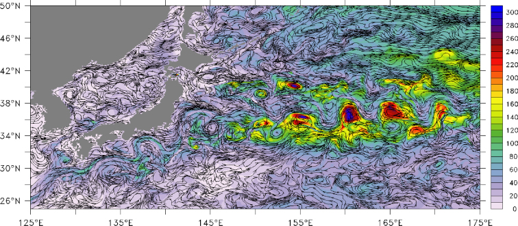
Figure 1. Snapshot of the high-resolution (0.1°) model field, taken at the end of the tracer injection period (end of April, model year 0): shading indicates the thickness of the surface mixed layer (in m); contouring illustrates the surface velocity field indicated by local stream lines.
Download figure:
Standard image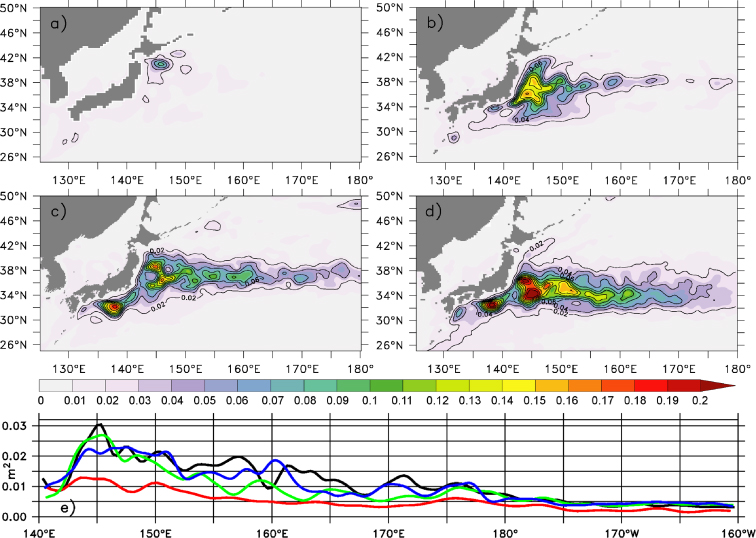
Figure 2. Variance of sea surface height during 1998–2007 (in m2; contour lines indicate a 0.02 m2 interval) from (a) 0.5°-model, (b) 0.25°-model, (c) 0.1°-model, (d) satellite altimeter data (AVISO) and (e) in a comparison along the axis of the Kuroshio extension (meridionally averaged between 32°N and 40°N), for AVISO data (black), the 0.5° (red), 0.25° (green) and 0.1° (blue) model simulations.
Download figure:
Standard image3.2. Initial tracer spreading
During the first weeks and months after release the tracer spreading is governed by the distribution of individual currents and eddies straddling the northern rim of the Kuroshio, giving rise to elongated streaks of high tracer concentrations (figures 3 and A.1). As indicated by low concentration values south of the Kuroshio axis (∼36°N), the Kuroshio acts as a barrier for the direct southward penetration of tracer, in line with ship-based observations provided by Buesseler et al (2012). The initial streakiness becomes smeared out after a few months (6–12) under the cumulative effect of eddies, resulting in a broadening tracer patch that appears to be drawn out into the central North Pacific by the mean eastward current system. Beside this preferred eastward propagation, some tracer fraction propagates to the northeast, reaching the southern portion of the Bering Sea after ∼3 years (figure 4(b)); another portion becomes drawn into the anticyclonic recirculation south of the Kuroshio, after reaching longitudes where the blocking effect of the Kuroshio becomes weaker (east of ∼155°E). After ∼7 months (figures 3(c) and (d)) the peak surface concentrations are diluted to less than 1% of the values in the coastal box at the end of the discharge period.
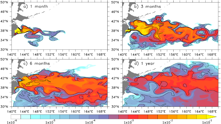
Figure 3. Sequence of relative surface tracer concentration during the first year from the 0.1° model simulation; contour lines mark power of 10 intervals.
Download figure:
Standard image
Figure 4. Decadal evolution of relative surface tracer concentration in the 0.1°-model simulation; boxes in (d) indicate regions for which the temporal evolution is computed in figure 7; contour lines mark power of 10 intervals.
Download figure:
Standard imageTo assess the importance of the local ocean state during and after the discharge period, the 0.25°-reference experiment was repeated by two 0.25°-cases with different initial states, i.e., the mid-March conditions of two other, arbitrarily chosen years. Temporal sequences of relative surface concentrations for the three cases are shown in figure A.1: they confirm the importance of the initial current distribution for the tracer spreading during the first months after injection, but indicate their relevance to fade for the longer-term tracer evolution. In all cases, the bulk of the total tracer inventory is flushed out of the western boundary region (30°–45°N, 140°–160°E) within 2–3 years (figure A.2). Peak concentrations for certain selected regions in the North Pacific (as discussed for the 0.1° model simulation, e.g. in figure 7) from the different sensitivity simulations occur within 1 year times span and are of the same magnitude.
3.3. Decadal tracer spreading
The subsequent evolution of the tracer distribution over the next years illuminates the combined effect of mean currents and eddies (figure 4). After one year the main tracer patch already extends beyond the dateline, with leading edges near 33°N and 45°N, apparently associated with the different branches of the Kuroshio Extension system that emerges to the east of the Shatsky Rise around 160°E (cf Niiler et al 2003). Tracer dispersion due to lateral eddy mixing and vertical mixing (see below) has by then led to a dilution of maximum surface concentrations by a factor of ∼500, and a broad cloud (with relative surface concentrations of 5 × 10⁻⁴–5 × 10⁻³) already covers a considerable fraction of the western Pacific basin between 27°N and 50°N. In the following years, the tracer cloud continuously expands laterally, with maximum concentrations in its central part heading east. While the northern portion is gradually invading the Bering Sea, the main tracer patch reaches the coastal waters of North America after 5–6 years, with maximum relative concentrations ( > 1 × 10⁻⁴) covering a broad swath of the eastern North Pacific between Vancouver Island and Baja California. Simultaneously some fraction of the southern rim of the tracer cloud becomes entrained in the North Equatorial Current (NEC), resulting in a westward extending wedge around 20°N that skirts the northern shores of the Hawaiian Archipelago. After 10 years the concentrations become nearly homogeneous over the whole Pacific, with higher values in the east, extending along the North American coast with a maximum (∼1 × 10⁻⁴) off Baja California. The southern portion of the tracer cloud is carried westward by the NEC across the subtropical Pacific, leading to increasing concentrations in the Kuroshio regime again.
The vertical penetration of the tracer appears strongly governed by the vigorous mixing processes associated with the O(200 m)-deep convection along the Kuroshio in the western North Pacific during episodes of wintertime cooling (Suga et al 2004). Since the tracer release took place near or just after the period of deepest surface mixed layer at the end of winter (figure 1), the simulation suggests a rapid penetration of the tracer into the upper 500 m of the water column already in the first weeks during and after injection (figure 5). The vertical mixing effect thus appears as a leading factor for the overall tracer dilution during the first and second year, i.e., as long as a significant fraction of the tracer has remained in areas where deep winter mixing takes place.
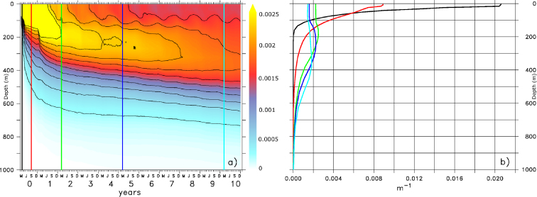
Figure 5. (a) Temporal evolution of relative vertical tracer distribution (in m−1), horizontally integrated over the North Pacific, from the 0.1°-simulation, contour lines mark a 2.5 × 10⁻⁴ interval; (b) vertical profiles from (a) after 15 days (black), 90 days (red), 2 years (green), 5 years (blue) and 10 years (light blue).
Download figure:
Standard imageThe effect of the explicitly resolved mesoscale eddies on the lateral tracer dispersion is elucidated in figure 6, showing the relative tracer concentration for the upper 1000 m (vertical integral) after 5 years for different model cases. While the mean eastward spreading of the main tracer patch appears as a robust feature of all model versions, there are some differences in the dispersion characteristics. The cloud has remained tightest and peak concentrations highest in the 0.5°-simulation. In the 'eddying' experiments the tracer has more effectively dispersed, especially in zonal direction where concentrations both near the western and eastern boundaries are significantly enhanced compared to the 0.5°-case. Peak concentrations in the 0.25°-case have become an order-of-magnitude smaller, and slightly decrease further in the 0.1°-case. Compared to the effect of resolution, a change in release duration (14 versus 54 days) is of negligible importance for the horizontal distribution.
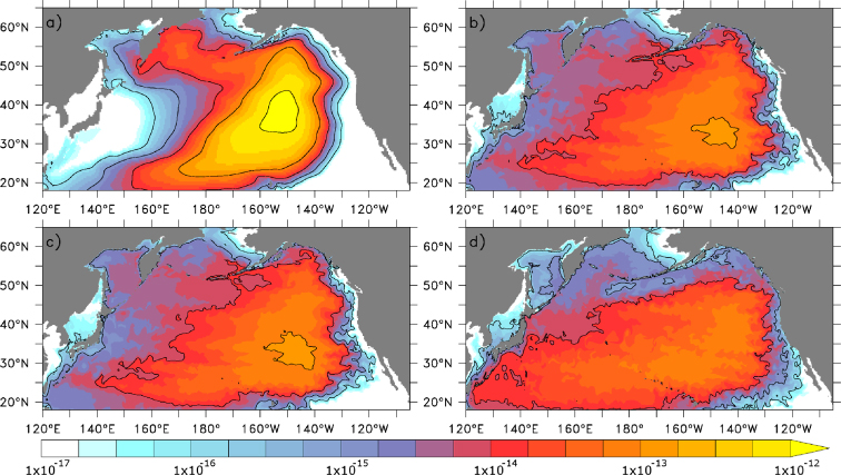
Figure 6. Effect of model resolution and discharge period on relative tracer concentration for the upper 1000 m (in m−2, vertical integral, relative to the tracer inventory in the upper 1000 m, area-standardized) after 5 years for (a) 0.5°-simulation (14 day release period), (b) 0.25°-simulation (14 day release period), (c) 0.25°-simulation (54 day release period), (d) 0.1°-simulation (54 day release period); contour lines mark power of 10 intervals.
Download figure:
Standard imageAs a quantitative measure of the dispersion effect the temporal evolution of the peak value of the relative concentration for each simulation (figure A.3) was compared. These results show much higher peak concentrations for the coarse 0.5°-case during the entire integration period, indicating an underestimation of the lateral mixing by the eddy parameterization. The differences between the higher-resolution models are comparatively small.
The temporal evolution of the peak tracer concentration in the 0.1°-simulation for a number of selected regions across the North Pacific (see figure 4(d) for area definitions) is shown in figure 7. For this analysis the relative tracer concentrations have been converted to absolute radioactivity values, by calibrating the total model inventory at the end of the discharge period with a tentative choice (10 PBq) for the total 137Cs deposition during the first weeks after the incident (Kawamura et al 2011). The estimated radioactivity values of the simulation can then be compared, e.g., to the pre-Fukushima 'background' radiation level, i.e. the remnant of previous nuclear weapon tests in the 1960s and the Chernobyl disaster in 1986, a level of about ∼1–2 Bq m−3 (e.g., Buesseler et al 2011, Hirose and Aoyama 2003; see also http://www.whoi.edu/page.do?pid=83397&tid=3622&cid=94989).
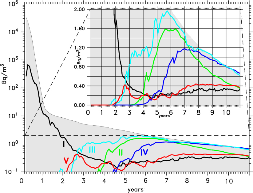
Figure 7. Temporal evolution of absolute peak concentrations (in Bq m−3, logarithmic scale; grey shaded) and within individual regions (see figure 4(d)) from the 0.1°-model simulation, assuming a total input of 10 PBq of 137Cs. Regions: western Pacific (I, black), off North America (II, green), Hawaii Islands (III, light blue), off Baja California (IV, blue), Aleutian Islands (V, red). The inset is a zoom into the part of the figure with levels below 2 Bq m−3 (pre-Fukushima values) on a linear scale.
Download figure:
Standard imageThe peak concentration at the end of the discharge period obtained in this way is 2–3 × 10⁴ Bq m−3; it represents the initial area-mean concentration for a coastal box of ∼9 km × 9 km within the input area, and is broadly consistent with the (sparse) offshore measurements during April 2011 made publicly available (see e.g. Buesseler et al 2011). The peak tracer concentration rapidly declines, by more than 3 orders of magnitudes, during the first year, reflecting the combined effect of vigorous eddy dispersion and vertical mixing in the western North Pacific. The pace of dilution becomes much more gradual thereafter, when the core of the tracer cloud is being advected to the central and eastern North Pacific; it thus takes 6–9 years to reduce the peak concentrations of the additional radioactivity to values comparable to the pre-Fukushima background levels (implying total values of about twice the pre-Fukushima level). During this period, the signal of peak tracer values approaches the North American continent, reaching the coastal area (Region II) after ∼5 years, with maximum values of ∼1.5 Bq m−3 on top of the background level. An even earlier (3–6 years) occurrence is obtained for the waters around Hawaii (Region III), with a peak of additional radioactivity of ∼2 Bq m−3. Peak values off Baja California (Region IV) are reached after 7 years (∼1 Bq m−3). The concentration around the Aleuts (Region V) begins to rise earlier, after about ∼2.5 years, by the direct meridional spreading; a second period of rising values starts upon the arrival of contaminated water with the cyclonic circulation along the North American coast.
3.4. Caveats
The interpretation of the simulated 'dye' tracer in terms of the actual 137Cs contamination needs to account for at least three major assumptions and idealizations. (1) The simulations do neither include an attempt to estimate the actual state of the local oceanic conditions off Japan during spring 2011, nor do they capture the small-scale coastal currents and tidal motions which governed the initial spreading phase as elucidated by Kawamura et al (2011): without such initialization (and without knowledge of the actual and future atmospheric forcing conditions), the simulations cannot give a deterministic account (nor a forecast) of the tracer spreading. On the other hand, the results from ensembles with varied initial conditions as reported by Dietze and Kriest (2011) and as performed here, lend some confidence to the assumption that the impact of the initialization would largely fade after the first 2–3 years. (2) The configuration of the tracer injection was set up primarily to capture the direct oceanic injection from the stricken power plants, whereas no explicit attempt was made to cover the atmospheric fallout that occurred over a wider, but not precisely known area of the western Pacific (Stohl et al 2012, Kawamura et al 2011); however, the choice of a non-local input area (150 km × 45 km) instead of a local oceanic injection (primarily to mimic the mixing effect of non-resolved near-coastal currents and tides), might be thought to possibly also capture some fraction of the atmospheric deposition in the vicinity of Fukushima. (3) The simulations neglected biological processes, e.g. adhesion to sinking particles, which could contribute to a more effective vertical mixing than by physical processes alone (Dietze and Kriest 2011).
4. Conclusions
The Pacific Ocean is a vast place, stirred by energetic, fluctuating currents on various scales, all contributing to an effective dilution of the contaminated body of sea water arising from the localized, idealized short-term discharge from the stricken Dai-ichi NPPs. The goal of the present study is to provide a clearer perspective of the spatio-temporal evolution of that dilution process over a decadal time span for a tracer corresponding to 137Cs injected over a near-coastal region off northeastern Japan. The fate of that dye (with a half-life corresponding to 137Cs) was examined by a host of simulations with a set of ocean circulation models differing in the representation of mesoscale eddy fluxes. With caution given to the various idealizations (unknown actual oceanic state during release, unknown release area, no biological effects included, see section 3.4), the following conclusions may be drawn. (i) Dilution due to swift horizontal and vertical dispersion in the vicinity of the energetic Kuroshio regime leads to a rapid decrease of radioactivity levels during the first 2 years, with a decline of near-surface peak concentrations to values around 10 Bq m−3 (based on a total input of 10 PBq). The strong lateral dispersion, related to the vigorous eddy fields in the mid-latitude western Pacific, appears significantly under-estimated in the non-eddying (0.5°) model version. (ii) The subsequent pace of dilution is strongly reduced, owing to the eastward advection of the main tracer cloud towards the much less energetic areas of the central and eastern North Pacific. (iii) The magnitude of additional peak radioactivity should drop to values comparable to the pre-Fukushima levels after 6–9 years (i.e. total peak concentrations would then have declined below twice pre-Fukushima levels). (iv) By then the tracer cloud will span almost the entire North Pacific, with peak concentrations off the North American coast an order-of-magnitude higher than in the western Pacific.
Acknowledgments
The model integrations were performed at the North-German Supercomputing Alliance (HLRN) and the computing centre at Kiel University. We gratefully acknowledge the support of the DRAKKAR group in model development. We further like to thank the developers of the freely available Ferret program used for analysis and graphics, provided by NOAA Pacific Marine Environmental Laboratory, available at www.ferret.noaa.gov. The altimeter products were produced by Ssalto/Duacs and distributed by Aviso, with support from Cnes (www.aviso.oceanobs.com/duacs/).
Appendix:

Figure A.1. Sequence of relative surface tracer concentration during the first 2 years, from 0.25° model simulations, differing in the initial year of the tracer release; contour lines mark power of 10 intervals.
Download figure:
Standard image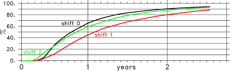
Figure A.2. Total fraction of tracer (in %) outside the western boundary region (30°N to 45°N, 140°E to 160°E, box marked in figure A.1) from three 0.25° model simulations, differing in the initial year of the tracer release.
Download figure:
Standard image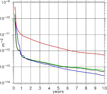
Figure A.3. Temporal evolution of the peak values for the relative tracer concentration in the upper 1000 m (in m−2, vertical integral, relative to the tracer inventory in the upper 1000 m, area-standardized): peak concentrations reach values between 6 × 10⁻¹¹ and 5 × 10⁻⁹ m−2 right after the injection period, highest in the 0.5° simulation (red). These values rapidly drop during the first year independent from the model's resolution. The decline then slows down, faster in the coarse case than in the eddying simulations where rather no difference is observed neither between the 0.25° (black) and 0.1° (blue) simulations nor between two 0.25° experiments differing in the release period (green: 14 days; black: 54 days).
Download figure:
Standard image