
Abstract
Sound policies for protecting coastal communities and assets require good information about vulnerability to flooding. Here, we investigate the influence of sea level rise on expected storm surge-driven water levels and their frequencies along the contiguous United States. We use model output for global temperature changes, a semi-empirical model of global sea level rise, and long-term records from 55 nationally distributed tidal gauges to develop sea level rise projections at each gauge location. We employ more detailed records over the period 1979–2008 from the same gauges to elicit historic patterns of extreme high water events, and combine these statistics with anticipated relative sea level rise to project changing local extremes through 2050. We find that substantial changes in the frequency of what are now considered extreme water levels may occur even at locations with relatively slow local sea level rise, when the difference in height between presently common and rare water levels is small. We estimate that, by mid-century, some locations may experience high water levels annually that would qualify today as 'century' (i.e., having a chance of occurrence of 1% annually) extremes. Today's century levels become 'decade' (having a chance of 10% annually) or more frequent events at about a third of the study gauges, and the majority of locations see substantially higher frequency of previously rare storm-driven water heights in the future. These results add support to the need for policy approaches that consider the non-stationarity of extreme events when evaluating risks of adverse climate impacts.
Export citation and abstract BibTeX RIS
1. Introduction
In coming centuries, multi-metre sea level rise (SLR) threatens permanent submersion or displacement of extensive coastal land, infrastructure and ecosystems (Overpeck et al 2006, Titus et al 1991, Wu et al 2009). In coming decades, smaller amounts of SLR will still impact low-lying coastal areas by augmenting the water levels reached by storm surges. The frequency of surges currently reaching a given height will thus increase (Kirshen et al 2008, Cooper et al 2008). Equivalently, the water level associated with any given frequency will grow, and communities should expect to see waters reach progressively new heights. These trends will very likely force changes in risk assessments related to extreme events (Hunter 2011), such as the delineation of 100 yr floodplains, that influence coastal policy and development (see for example a recent circular by the US Army Corp of Engineers setting forth guidelines for the consideration of SLR qualitatively consistent with our approach: http://140.194.76.129/publications/eng-circulars/EC_1165-2-212_2011Nov/EC_1165-2-212_2011Nov.pdf).
In this letter, we develop projections through mid-century of SLR-driven changes in the return periods (or equivalently levels) of extreme storm surges, for a network of coastal tide gauge stations in the contiguous United States. First, we estimate the historical SLR rate at each gauge, and use it to detrend the gauge's hourly records. We then analyse extreme annual values in these adjusted records, on the basis of daily maximum observed water levels. These represent our best estimates of current storm surge statistics, conditional on the observed combination of weather and tidal components. We use the peak-over-threshold approach from extreme value theory, fitting generalized Pareto distributions to threshold exceedances.
After determining baseline return levels at each gauge for several representative return periods spanning between 1 and 100 yr, we add near- and mid-term projections (respectively, by 2030 and 2050) of the relative SLR at the gauge, and compare the resulting future return level curves against baseline. We derive our relative SLR projections from a semi-empirical model of global sea level recently proposed by Vermeer and Rahmstorf (2009), whose results we modify locally by using our gauge-specific estimates of historic relative SLR.
The overall analysis combines best estimates and ranges of uncertainty for each of the terms into an assessment of the likely range of outcomes.
2. Data and procedure
We use hourly and monthly records from 55 tide gauge stations (see table 1), distributed along the coasts of the contiguous United States (see map in figure 2). For all these stations, we have time series of observed water levels and predicted ones (i.e. produced by the National Oceanic and Atmospheric Administration (NOAA) based only on tides and seasonal cycle). We have registered these values to each location's mean high water (MHW) datum (see http://tidesandcurrents.noaa.gov/datum_options.html for an explanation of tidal datums). The records are not complete, but the 55 selected gauges have less than 10% of missing values over the 30 yr hourly data period, 1979–2008, and an even lower fraction of missing monthly data over the 50 yr period spanned by the monthly record, 1959–2008.
Table 1. Current trend at each gauge in mm yr−1 (column 1); expected value (ensemble mean) of relative sea level rise by 2030 and 2050 (reference year: 2008) in metres (columns 2 and 3); 50- (column 4) and 100- (column 5) yr return levels of storms in metres above MHW where MHW is computed according to the gauge epoch, generally 1983–2001. The trend for gauge 8772440 (Freeport, TX) has been computed allowing for an unknown offset starting on 1st January 1972, likely due to a change in the primary benchmark. The revised value of the trend is significantly smaller than what would be fitted by a simple linear regression over the time series' length. Additionally we used the smallest estimate of a 30 yr trend within the 50 yr available for the gauges identified by an apostrophe next to their numbers (see discussion in section 2.2 and supplementary material available at stacks.iop.org/ERL/7/014032/mmedia). For reference we add a line showing global trends and sea level rise projections estimated by the ensemble mean of the simulations available, after inputting them individually into the semi-empirical model and averaging the annual rates so derived over the respective reference periods.
| Station | 1959–2008 trends (mm yr−1) | SLR 2008–30 (m) | SLR 2008–50 (m) | 50 yr RL (m) | 100 yr RL (m) | |
|---|---|---|---|---|---|---|
| 8410140 | Eastport, Passamaquoddy Bay, ME | 0.96 | 0.09 | 0.24 | 1.56 | 1.64 |
| 8418150 | Portland, Casco Bay, ME | 1.10 | 0.10 | 0.25 | 1.14 | 1.19 |
| 8443970 | Boston, Boston Harbor, MA | 2.31 | 0.12 | 0.30 | 1.50 | 1.66 |
| 8447930 | Woods Hole, Buzzards Bay, MA | 2.63 | 0.13 | 0.31 | 1.28 | 1.42 |
| 8449130 | Nantucket Island, Nantucket Sound, MA | 2.96 | 0.14 | 0.32 | 1.17 | 1.29 |
| 8452660 | Newport, Narragansett Bay, RI | 2.64 | 0.13 | 0.31 | 1.24 | 1.40 |
| 8454000 | Providence, Providence River, RI | 2.15 | 0.12 | 0.29 | 2.03 | 2.54 |
| 8461490 | New London, Thames River, CT | 2.58 | 0.13 | 0.31 | 1.16 | 1.22 |
| 8467150 | Bridgeport, Bridgeport Harbor, CT | 2.37 | 0.12 | 0.30 | 1.50 | 1.66 |
| 8510560 | Montauk, Fort Pond Bay, NY | 3.23 | 0.14 | 0.34 | 1.16 | 1.24 |
| 8518750 | The Battery, New York Harbor, NY | 2.87 | 0.14 | 0.32 | 1.40 | 1.53 |
| 8534720 | Atlantic City, Atlantic Ocean, NJ | 4.42 | 0.17 | 0.39 | 1.39 | 1.52 |
| 8536110 | Cape May, Cape May Canal, Delaware Bay, NJ | 4.02 | 0.16 | 0.37 | 1.27 | 1.37 |
| 8551910 | Reedy Point, C&D Canal, DE | 3.67 | 0.15 | 0.35 | 1.04 | 1.14 |
| 8557380 | Lewes, FT. Miles, DE | 3.31 | 0.15 | 0.34 | 1.45 | 1.58 |
| 8571892 | Cambridge, Choptank River, MD | 3.26 | 0.14 | 0.34 | 1.06 | 1.20 |
| 8574680 | Baltimore, Fort McHenry, Patapsco River, MD | 2.94 | 0.14 | 0.32 | 1.43 | 1.69 |
| 8575512 | US Naval Academy, Severn R., Ches. Bay, MD | 3.08 | 0.14 | 0.33 | 1.32 | 1.55 |
| 8577330 | Solomons Island, Patuxent River, MD | 3.93 | 0.16 | 0.37 | 1.08 | 1.27 |
| 8594900 | Washington, Potomac River, DC | 3.09 | 0.14 | 0.33 | 2.31 | 3.01 |
| 8632200 | Kiptopeke, Chesapeake Bay, VA | 3.57 | 0.15 | 0.35 | 1.07 | 1.13 |
| 8635750 | Lewisetta, Potomac River, VA | 4.98 | 0.18 | 0.41 | 1.05 | 1.20 |
| 8638610 | Sewells Point, Hampton Roads, VA | 4.76 | 0.18 | 0.40 | 1.44 | 1.57 |
| 8638863 | Chesapeake Bay Bridge Tunnel, VA | 5.72 | 0.20 | 0.44 | 1.28 | 1.36 |
| 8656483 | Beaufort, Duke Marine Lab, NC | 3.09 | 0.14 | 0.33 | 1.20 | 1.45 |
| 8658120 | Wilmington, Cape Fear River, NC | 2.18 | 0.12 | 0.29 | 1.02 | 1.17 |
| 8661070 | Springmaid Pier, Atlantic Ocean, SC | 3.98 | 0.16 | 0.37 | 1.08 | 1.17 |
| 8665530 | Charleston, Cooper River Entrance, SC | 3.00 | 0.14 | 0.33 | 1.28 | 1.51 |
| 8670870 | Fort Pulaski, Savannah River, GA | 3.33 | 0.15 | 0.34 | 0.92 | 0.95 |
| 8720030 | Fernandina Beach, Amelia River, FL | 2.44 | 0.13 | 0.30 | 0.93 | 0.97 |
| 8723970 | Vaca Key, Florida Bay, FL | 3.02 | 0.14 | 0.33 | 0.71 | 0.86 |
| 8724580 | Key West, FL | 2.60 | 0.13 | 0.31 | 0.74 | 0.90 |
| 8725110 | Naples, Gulf of Mexico, FL | 2.09 | 0.12 | 0.29 | 1.04 | 1.16 |
| 8726520 | St Petersburg, Tampa Bay, FL | 2.68 | 0.13 | 0.31 | 1.57 | 1.94 |
| 8726724 | Clearwater Beach, Gulf of Mexico, FL | 2.30 | 0.12 | 0.30 | 1.58 | 1.97 |
| 8728690 | Apalachicola, Apalachicola River, FL | 1.28 | 0.10 | 0.25 | 3.15 | 4.53 |
| 8729840 | Pensacola, Pensacola Bay, FL | 2.04 | 0.12 | 0.29 | 2.76 | 4.20 |
| 8761724' | Grand Isle, East Point, LA | 6.49 | 0.22 | 0.47 | 1.99 | 2.78 |
| 8770570' | Sabine Pass North, TX | 2.17 | 0.12 | 0.29 | 1.52 | 1.89 |
| 8771450' | Galveston Pier 21, Galveston Channel, TX | 4.92 | 0.18 | 0.41 | 1.69 | 2.08 |
| 8771510' | Galveston Pleasure Pier, Gulf of Mexico, TX | 6.06 | 0.21 | 0.45 | 2.51 | 3.38 |
| 8772440' | Freeport, Dow Barge Canal, TX | 3.48* | 0.15 | 0.35 | 1.39 | 1.59 |
| 8774770' | Rockport, Aransas Bay, TX | 3.65 | 0.15 | 0.35 | 1.37 | 1.84 |
| 8779770' | Port Isabel, Laguna Madre, TX | 3.16 | 0.14 | 0.33 | 1.33 | 1.74 |
| 9410230 | La Jolla, Pacific Ocean, CA | 2.12 | 0.12 | 0.29 | 0.94 | 0.95 |
| 9410660 | Los Angeles, Outer Harbor, CA | 1.15 | 0.10 | 0.25 | 0.94 | 0.96 |
| 9412110 | Port San Luis, Pacific Ocean, CA | 0.40 | 0.08 | 0.22 | 1.01 | 1.06 |
| 9413450 | Monterey, Monterey Harbor, CA | 1.03 | 0.10 | 0.24 | 0.98 | 1.03 |
| 9414290 | San Francisco, San Francisco Bay, CA | 1.74 | 0.11 | 0.27 | 1.13 | 1.23 |
| 9432780 | Charleston, Coos Bay, OR | 0.92 | 0.09 | 0.24 | 1.29 | 1.33 |
| 9435380 | South Beach, Yaquina River, OR | 2.29 | 0.12 | 0.30 | 1.31 | 1.37 |
| 9439040 | Astoria, Tongue Point, Columbia River, OR | −0.29 | 0.07 | 0.19 | 1.34 | 1.36 |
| 9440910 | Toke Point, Willapa Bay, WA | 1.09 | 0.10 | 0.25 | 1.85 | 1.96 |
| 9443090 | Neah Bay, Strait of Juan de Fuca, WA | −2.06 | 0.03 | 0.11 | 1.44 | 1.47 |
| 9447130 | Seattle, Puget Sound, WA | 1.83 | 0.11 | 0.28 | 1.20 | 1.23 |
| 0000000 | Global | 2.89 | 0.14 | 0.32 |
2.1. Current trend and extreme value analysis
Our analysis begins with factoring out SLR from observed gauge water levels. We fit the 50 yr record of monthly data at each gauge with a linear model, and use it to detrend the 30 yr hourly series, preserving its mean at MHW for the current national tidal datum epoch. This epoch is for a majority of gauges 1983–2001, but in Louisiana and Texas most gauges have been assigned more recent 5 yr epochs to keep up with that coastal region's rapid subsidence.
Sea level trends vary geographically, even in sign, as table 1 details. The largest estimates are found in the Gulf of Mexico and the mid-Atlantic. The smallest values are in the Pacific Northwest, where at two gauges the trend is actually negative, a phenomenon mainly due to local uplift of the continental shelf (Mazzotti et al 2008).
The detrended values quantify the effects of day-to-day weather, tides and seasonal cycles on water level and form the basis for our extreme value analysis. From the hourly values we compute daily maxima and perform a peak-over-threshold (POT) analysis by selecting, after trial and error, a threshold corresponding to the 99th percentile of each gauge's distribution of observed water levels. This choice ensures that the threshold falls above NOAAs highest predicted levels based on tides and seasons alone. In each time series, we then identify those daily values exceeding the threshold, also requiring that successive exceedances be at least one day apart, and taking only the maximum from among consecutive extremes. Given these measures, exceedances from the same storm should not be counted as independent events.
On the basis of these exceedance values and their frequency of occurrence each year, we fit the parameters of a generalized Pareto distribution (GPD), which models the distribution function of exceedances by the form

where u is the value of the threshold,  and the parameters μ, σ and ξ control the location, scale and shape of the distribution. This part of the analysis essentially extends what Zervas (2005) showed, except here we use the POT approach and thus a GPD model rather than the generalized extreme value distribution approach; and we use daily rather than monthly data. Note also that a recent paper (Menéndez and Woodworth 2010) analysed POT at a global network of gauges utilizing longer records and allowing the parameters of the GPD to vary over time. Here we assume that in this relatively shorter time period of 30 yr and after the elimination of the long-term trend, which would likely influence the value of the location parameter of the GPD, the extreme behaviour can be approximated through a fixed set of parameters. Our motivation also stems from the awareness that robust estimates of time-varying parameters of extreme value distributions are a challenge even when based on longer records (Coles 2001).
A simple functional relation links the parameters of the GPD to measures of return levels and return periods, which we therefore compute after estimating the values of the GPD parameters by maximum likelihood.
2.2. Sea level rise projections
We proceed now to incorporate the component of near- (2030) and mid-term (2050) future SLR. We begin by considering global SLR projections. Many variables will influence and contribute to uncertainty around global mean sea level this century, including the future trajectory of greenhouse gas emissions; the response of atmospheric and oceanic temperatures to these; and the melting and dynamic collapse of glaciers and ice sheets in response to changing temperatures (Meehl et al 2007). Numerical models' simulations of sea level rise, however, especially at regional scales, are not mature enough, yet, to justify their direct use, showing inconsistencies with observed patterns and large differences in the projected ones (Gregory et al 2001, Meehl et al 2007). They are also limited to the thermal expansion component of the rise, as they do not represent the processes leading to ice sheet melting and collapse.
Here we instead adopt the semi-empirical approach of Vermeer and Rahmstorf (2009), VR09 from now on. The method relies on estimates from observations and model simulations of the coefficients of a linear relationship between the rate of sea level rise at time t,  , the global warming from a reference period T − T0 and a measure of instantaneous global warming,
  , as in:

The coefficients a and b can then be applied to climate model simulations of future global temperature change to infer projections of global SLR. Note that with this semi-empirical approach, VR09 implicitly incorporates both terrestrial ice loss and thermal expansion of warming water. We choose to adopt this method because of the relatively short-term nature of our analysis, out to 2050, that makes VR09's reliance on extrapolation more defensible, coupled with our need for a method that allowed uncertainty characterization at a reasonable computational cost. We can incorporate therefore uncertainty from emissions scenarios and climate models' different sensitivities by using an ensemble of trajectories of future global warming spanning a range of greenhouse gas emission pathways and climate models' parameters. The robustness of the projections obtained by the VR09 method has been recently documented in Rahmstorf et al (2011).
Additional factors add variation and compound uncertainties with respect to regional and local projections of sea level rise. These include vertical land motion from glacial isostatic adjustment and other causes, ocean thermal expansion, shifting currents, and gravitational effects, all detailed at greater length in the supplementary material (available at stacks.iop.org/ERL/7/014032/mmedia). Our approach to deriving SLR projections for each gauge location uses historical information to derive the local component of observed SLR that can be most robustly characterized as having a long timescale. By using linear trends over 50 yr of data, a long established standard (Roemmich 1990, Douglas 1992), we aim at cancelling out the effect of local interdecadal oscillations from variable currents and other dynamic factors. An analysis of the trends and their residuals after removal of independently measured vertical land motions supports this approach, and thus the extrapolation forward of the local component, for most gauges, with the exception of those located in the western Gulf of Mexico (see supplementary material available at stacks.iop.org/ERL/7/014032/mmedia). There, high and spatiotemporally variable subsidence rates likely linked to subsurface oil, gas and water extraction call into question the robustness of any linear fit to the record. In fact, the behaviour of 20- and 30 yr trends at these gauges shows the largest variability within the 50 yr record of all gauges in the dataset. Western Gulf SLR is also highest in the dataset when characterized as the 50 yr trend, while fits applied to the last 20 or 30 yr estimate a slower rise. Given the strong apparent effects of subsurface fluid extraction and the highly nonlinear data for these gauges, we choose to characterize the local component for Texas and Louisiana gauges in a conservative manner, adopting the smallest value among the 30 yr trends derived by a sliding window over the 50 yr history. In doing so we attempt to approximate a 'baseline rate' little or not affected by extraction, since extraction activities may diminish or cease over the future time horizon of our analysis. We mark the gauges where we adopt this arbitrary choice by an apostrophe in table 1.
When satisfied that the measures of relative SLR at all gauges are robust, or at least conservative, we can perform an extrapolation of the local component of SLR estimated over the last half century by coupling it to the global sea level rise projections produced by the semi-empirical global approach. Given the large uncertainties affecting local projections as derived directly from climate models (Meehl et al 2007, figure 10.32), and the short time horizon of our projections, we argue that our approximation should be considered an acceptable exercise. We ignore effects from projected shifts in Atlantic meridional overturning circulation (Yin et al 2009, 2010, Korper et al 2009, Lorbacher et al 2010) and gravitational fingerprints (e.g. Mitrovica et al 2011), but these should be small compared to other factors in the time period considered (see supplementary material available at stacks.iop.org/ERL/7/014032/mmedia).
Were we only to work with single best estimates of global sea level rise for historic and future changes, our method would be synthesized in this simple explanation: we would take the global sea level rise projections from VR09 (0.14 and 0.32 m by, respectively, 2030 and 2050, obtained as the ensemble mean from all simulations available) and, for each gauge, we would add a local delta term based on the observed relative sea level rise during the period 1959–2008 at the gauge minus the corresponding change obtained through VR09 over the same period (0.14 m, again obtained as the ensemble average change, using as input to the semi-empirical model simulations of global average temperature change over the period 1959–2008).
In analytical terms, and accounting for the characterization of uncertainty through the ensemble of simulations, our approach can be described in more detail as follows.
We assume that at each gauge i the long-term SLR lri is the result of a global average component, gr offset by a gauge-specific additive constant, Δi (mainly due to the constant effect, on the 50- to 100 yr timescale, of vertical land movement). This can be written as

where the subscript 0 refers to the historical period. We can then similarly model the future relative SLR as

where the subscript 1 refers to a time in the future.
VR09 allows us to derive estimates of gr1 on the basis of a number of model simulations exploring scenario and parameterization uncertainties. If over 1959–2008 these model simulations all reproduced exactly gr0, the historical rate of SLR, we would simply use observed gr0 in equation (3), and modelled gr1 in (4). However, all model simulations are expected to produce a biased response for the historic period, and we want to take that into account, thus applying a standard approach in future climate change projections. Therefore, rather than computing Δi as the difference of local and global observed rates, from equation (3), and applying that estimate in equation (4) to the modelled gr1, we compute an ensemble of  based on

where the superscript m refers to a model parameterization/scenario combination, and the ensemble of modelled historical rates are substituted for the observed rate. We then compute, accordingly, an ensemble of future rates as in

Simple algebraic manipulation shows that this is equivalent, under the assumption of an additive constant offset, to using observed gr0 in equation (5), and to bias-correcting  in (6), by the constant bias term calculated in the historic period as
  .
.
By utilizing the data made available through VR09, we are able to explore responses of global temperature as simulated from 19 different GCMs, under 6 different SRES scenarios and assuming three different parameterizations of the global carbon cycle. Note that given the near- to mid-term forecast horizon we are interested in, the separation between scenarios contributes less to the uncertainty range than it would for longer term projections. See figure 1 for a plot of modelled global temperature anomalies for our study period, which constitute the inputs to our SLR calculations through equation (2).

Figure 1. Simulated global temperature anomalies (compared to pre-industrial baseline, i.e., 1880 through 1920) which enter the computations of current and future rates of sea level rise according to VR09's semi-empirical model. Units of degrees C.
Download figure:
Standard image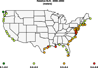
Figure 2. Sea level rise (mean estimate from 19 models temperature projections, under 6 scenarios and for 3 carbon cycle parameter settings) over the period 2008–50 at 55 tide gauges. Units of metres.
Download figure:
Standard imageFigure 2 shows the resulting mean SLR projections by 2050 (binned in 10 cm increments) while table 1 reports the actual estimates (in terms of ensemble averages). Obviously, on the basis of our assumptions, future SLR projections are larger where current trends are larger.
We can now proceed to superimpose future projections of sea level rise, together with their uncertainty bounds, on the estimated return levels and their uncertainty. In section 3, we present results for a set of gauges in terms of the change in return levels for periods of 1, 2, 10, 20, 30, 50, 75 and 100 yr. We compare estimates for the present to the 2030 and 2050 values obtained by adding sea level increases computed with respect to the current epoch's gauge datum. For a number of representative gauges we present separate results by including either uncertainty from the extreme value analysis alone, or together with SLR uncertainty, in order to assess the relative importance of these two sources.
We use the statistical software R (2004) to perform all computations, after translating into that language the MATLAB code provided by VR09. For the extreme value analysis we use the R package extRemes, available from http://cran.r-project.org/web/packages/extRemes/index.html.
3. Results and discussion
Figure 3 summarizes our GPD analysis results with best estimates (by maximum likelihood) for the 100 yr return levels of annual storm surges, a common benchmark for planning and vulnerability analysis, based on the detrended observed values at each gauge. Gulf region storm surges are in absolute terms largest; since the gauge records in our analysis include the effects of tropical cyclones, this is no surprise. Conversely, among the three coasts, Pacific extremes are generally smallest, due to the absence of hurricanes and of a wide, shallow continental shelf. Local characteristics also appear to play a role. Gauges near the margins of continental shelves (e.g. in the Florida Keys) may see low surges compared to those in areas behind wide shelf zones. Gauges deep in estuaries (e.g. in the Potomac River) may see relatively high surges if there is a strong river influence or if the shape of the estuary favours amplification of surge waters from the prevailing storm direction. Results in areas subject only with low probability to tropical cyclones will vary according to whether or not gauges experienced significant hits during our 30 yr reference period (e.g., the gauges at Georgia's corners did not—in line with low cyclone activity in Georgia for the whole 20th century). See table 1 for the precise numerical estimates displayed here, but we want to highlight that decisions related to vulnerabilities to hurricane damage are better served by locally focused modelling studies (e.g., Lin et al 2010a, 2010b) complementing observationally based statistics, also because it is not to be expected that the fit of a single parametric distribution will do justice to the modelling in places where tropical cyclones create significant surges, and those are mixed in the records with the effect of synoptic weather patterns.
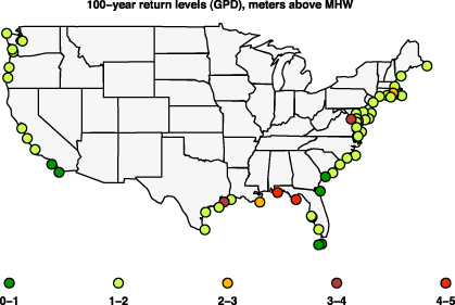
Figure 3. Maximum likelihood estimates of return levels, or heights, for 100 yr events. Units are metres above MHW, with MHW computed with respect to gauge epoch (1983–2001 for most gauges).
Download figure:
Standard imageObviously, sea level rise will add a positive offset to return levels everywhere. How quickly that offset increases the frequency of what would currently be a rare and extreme surge is our next concern. Figure 4 shows estimated future return periods for what today would be classified as '100 yr' events (return levels with 1% annual probability). Smaller estimates indicate larger changes. A few locations show no perceptible change by 2050 (grey dots), but for the great majority the return period is shortened considerably, even down to 1 yr, as indicated by the scatter of colours other than grey. Note that given the large uncertainty ranges surrounding estimates of each return level curve we choose to adopt a fairly coarse discretization of return periods. The delineation between bins used in figure 4 remains therefore fuzzy.

Figure 4. For the ensemble average estimate of relative SLR at each gauge, projected return periods, by 2050, for floods currently qualifying as 100 yr events.
Download figure:
Standard imageComparison to figure 3 shows a striking inverse relation when examining the geographic patterns of these frequency increases and the size of 100 yr events today. At the same time, the relationship to relative SLR rate (figure 2) is not as straightforward, highlighting the interplay between the amount of SLR and the size of current events in determining the change in frequency of rare events. Of course 'rare' does not coincide everywhere with 'of large magnitude', hence the need for locally focused assessment, taking into account not only the change in return period but also the size of the future event, in combination with local topography and patterns of development, before deeming these results significant from the perspective of practical risks.
We now focus on a representative subset of six gauges allowing cross-regional comparison of return level curves and their interactions with projected sea level rise, as shown in figure 5. (Results for all 55 gauges are available upon request from the first author.) In this figure we incorporate only ensemble mean SLR projections, corresponding to vertical offsets from the green curves. Therefore we show uncertainties pertaining only to the estimates of extreme behaviour. For two of the gauges, figure 6 further incorporates uncertainties from VR09, and so from emissions scenarios, carbon cycle modelling, climate model response, and the semi-empirical model response of SLR to global temperature, which being a fit in itself comes with uncertainty ranges.
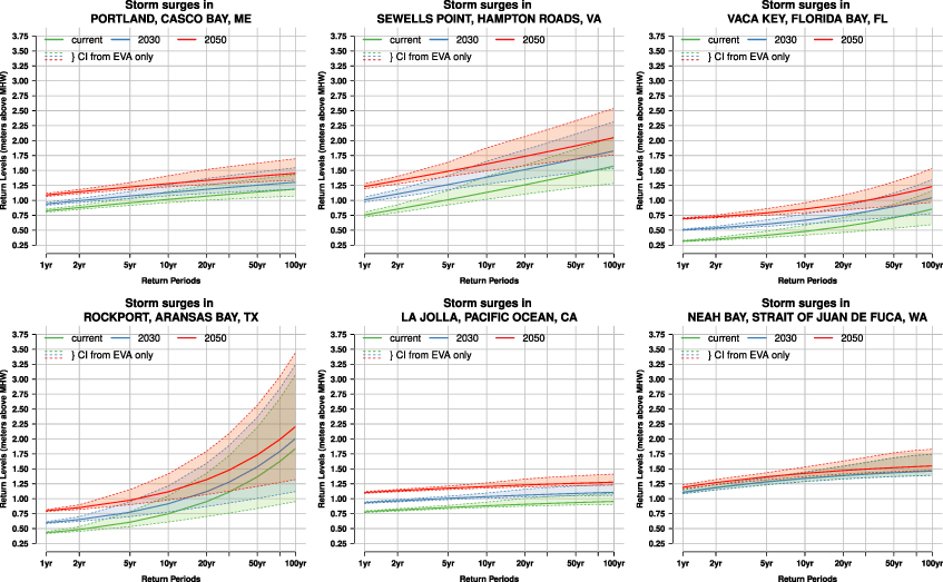
Figure 5. Return level curves for storm surges at six gauges exemplifying different behaviours along the US coasts. Estimates of uncertainties (95% confidence intervals) only from the extreme value analysis are included, depicted as shaded envelopes and dashed lines around the solid return level curves. Green curves and envelopes: estimates from observed record. Blue lines and envelopes: estimates incorporating projected relative SLR by 2030. Red lines and envelopes: estimates incorporating projected relative SLR by 2050.
Download figure:
Standard image
Figure 6. For two gauges among the six used in figure 5, we compare the uncertainty bounds when including confidence intervals only from the extreme value analysis (left panels, as in figure 5) and the uncertainty bounds when also including the uncertainty in sea level rise projections (right panels).
Download figure:
Standard imageWithin each plot in both figures, and reflecting each location's estimated relative SLR signal by 2030 and 2050, constant offsets separate the individual solid return level curves. This relation stems from our assumption that the characteristics of the extremes (i.e., the parameters of the GPD) remain constant in time, and only sea level changes. Note that we are not claiming confidence over the fact that the variability of storms will remain constant in the future. Rather, we work under the assumption that the dominant effect changing the frequency of flooding events will be mean sea level rise. This assumption is backed up by the two most recent IPCC reports (Church et al 2001, Meehl et al 2007) and, for example, Woodworth and Blackman (2004). The thickness of the shaded envelopes increases for longer return periods (along the x-axis dimension) due to the larger uncertainties in estimating rarer extremes, especially at gauges with steep curves (i.e., influenced by tropical cyclones). As shown in figure 6 the thickness also increases going from green to blue to red curves, due to the larger uncertainties in SLR projections as we increase the forecast horizon from present (no uncertainty) to 2030 and then 2050. Adding SLR uncertainties to extreme value analysis uncertainties generally appears to double the thickness of the shaded envelopes when considering intermediate return levels of one to a few decades. These confidence envelopes stake out a range of possibilities critical to policy considerations.
Focusing now on the solid lines (i.e., the maximum likelihood estimate) in figure 5, we can glean the main characteristics of storm surges and projected changes when comparing locations in very different regions of the US coast. The most striking aspects of these curves appear to be linked to the presence of tropical storms in the observed records of gauges in the Gulf of Mexico and lower- to mid-Atlantic. For these three gauges the curves are actually concave upward (their first derivative increasing for longer return periods), albeit almost imperceptibly so in the case of Sewells Point, due to the effect of very large values observed as their rarest events. It is easy to compare how different the behaviour is for locations where such extremes do not appear and the curve shapes are flatter and concave downward.
It is also easy to gauge—using the common range of the y-axis in these panels—that the curves show a large variation in their steepness (e.g., the difference between the left- and right-most points of each green curve). This variation across locations substantially exceeds the variation in projected local SLR by 2050 (the constant offsets between red and green curves). Accordingly, as already suggested, it appears that the shape of return level curves—more so than local SLR rates—will determine differentials in local exposure to higher water levels in coming decades, with locations characterized by flatter curves seeing the larger changes in return period for a given amount of sea level rise. This means that areas unaccustomed to significant storm surges (e.g. along the Pacific coast) should generally see the largest reductions in return periods for a given sea level rise. If this is also a significant change in flood risk will of course depends on the actual water height values and area topography and development patterns (see e.g. Strauss et al 2012). Therefore, adaptation planning will have to consider these nuances in order to assess if risks are changing seriously. Our general finding echoes a recent result from Mahlstein et al (2011), who found that local temperatures will depart from historical ranges faster in the tropics than in high latitudes, because lower tropical temperature variability will outweigh the slower warming there.
We performed the same overall analysis using 50 yr (rather than 100 yr) return levels as points of reference, and separately tried extending the study period through 2100. Both cases yielded qualitatively similar results to what we present here.
4. Conclusion
In this letter, we have combined information from historical tide gauge records of water level with estimates of future global sea level rise. We have analysed current local trends and storm surge return levels in order to project changes in future return levels and periods, while attempting to characterize uncertainties as fully as possible.
The extreme value theory framework allowed us to use a fairly short but high frequency and nearly complete record to provide estimates of return levels of storm surges—incorporating weather and tide effects—for multidecadal return periods, together with their uncertainties. We then incorporated semi-empirical estimates of sea level rise out to 2050, together with their confidence bounds. The latter have their main sources in models' uncertain projections of temperature increases over the same period and depend on an empirically fitted relation between temperature changes and sea level rise rates. An additional level of approximation has to be introduced when we use the difference between the historical rates of SLR as observed at the local and global scale and we apply a constant bias correction to future modelled rates to project future relative SLR.
A future approach to reducing some of this uncertainty, and extracting more information from the historical record, would be to disentangle the influence of tides from the historical water level record. This would substantially increase the signal-to-noise ratio in the storm record, and allow future projections to be made through the careful combination of separate storm surge and tide level probability distributions.
We also note that our model assumes that the nature of extreme water levels will remain constant in the future. Other studies have used dynamically modelled storm surges under different scenarios to assess possible future changes in the statistics of extremes for limited localities (see e.g. Cayan et al 2008, McInnes et al 2009, Purvis et al 2008). Of course, those studies also have to assume that the climate model representation of the future drivers of coastal storms is reliable, and we could refer to our discussion of the uncertainties in local sea level rise projections to defend the rationale for our 'all-else-being-equal' approach to characterizing the effects of SLR on high water events. Also, see Thompson et al (2009) for a comparison of statistical and dynamical approaches' pros and cons in an analysis focused on the Canadian North Atlantic coast. Other studies have looked at changes in statistical characteristics of observed storm surges, with mixed results. We already mentioned Menéndez and Woodworth (2010), where changes of the parameters of the extreme value distributions were found to be significant for locations around the globe, while more focused studies (e.g. Zhang et al 2000) do not support significant changes in storm intensity or frequency. Perhaps most importantly, at the base of this assumption is the consideration that the dominant effect over changing flood risks will be likely carried by mean water level changes rather than changes in storm variability. In this respect, however, we also need to point out that our approach does not account for the nonlinear effect of deeper water (higher mean sea levels) on storm surges created by a diminished bottom friction at locations along shallow coasts. This is also an effect that only dynamical models could address.
Finally, we want to stress that the estimates of sea level rise rates are based on model simulations that do not aim at representing natural low frequency (decadal) variability, albeit it could be argued that some of those low frequency variations are represented in the extreme value statistics. Model outputs thus show a smooth response to increased concentrations of greenhouse gases, to be interpreted as an average response rather than the precise behaviour of the Earth system at the exact dates represented in the simulation. This is similar to how projections of temperature change should be interpreted when obtained through climate model simulations. These projections do not attempt to forecast actual conditions on any given date, but rather represent average response over climatological (i.e., multidecadal) timescales.
Through this study we are able to offer a picture of likely changes in the return levels and periods of coastal storm surges in the next decades that, depending on the location, may significantly alter risk assessment related to high water levels and should be considered a relevant result for stakeholders and policy makers involved in coastal infrastructure or environmental protection decisions. Pacific coast locations are most in danger of seeing their historical extremes frequently surpassed in the coming few decades, followed by the Atlantic. Gulf locations appear in least danger of a rapid shift, despite rapid relative sea level rise, due to the high amplitudes of historical storm extremes, which render the relative effect of sea level rise small. The greater near term risk in the Gulf (as in a large portion of the Atlantic coast) is however the possibility of increasing cyclone intensity (Knutson et al 2010), concerns we do not address here. Our work provides further evidence that conducting risk assessments of coastal flood hazards must account for non-stationary behaviour, driven mainly by rising mean sea level.
Acknowledgments
The authors would like to thank two anonymous referees for their extensive feedback that greatly improved this study. They also thank the participants in the 2011 NCAR/ASP summer colloquium on extremes for productive discussions of this work; Richard Snay for guidance and supply of vertical land motion data; Robert Kopp, Jerry Mitrovica and Carling Hay for discussions and providing their gravity fingerprint model; M Ishii, Jianjun Yin and Ronald Stouffer for helpful correspondence concerning thermosteric effects. Claudia Tebaldi thanks the Climate and Global Dynamics Division, Climate Change Research Section at the National Center for Atmospheric Research in Boulder, CO, for hosting her.