

Abstract
Natural carbon sinks currently absorb approximately half of the anthropogenic CO2 emitted by fossil fuel burning, cement production and land-use change. However, this airborne fraction may change in the future depending on the emissions scenario. An important issue in developing carbon budgets to achieve climate stabilisation targets is the behaviour of natural carbon sinks, particularly under low emissions mitigation scenarios as required to meet the goals of the Paris Agreement. A key requirement for low carbon pathways is to quantify the effectiveness of negative emissions technologies which will be strongly affected by carbon cycle feedbacks. Here we find that Earth system models suggest significant weakening, even potential reversal, of the ocean and land sinks under future low emission scenarios. For the RCP2.6 concentration pathway, models project land and ocean sinks to weaken to 0.8 ± 0.9 and 1.1 ± 0.3 GtC yr−1 respectively for the second half of the 21st century and to −0.4 ± 0.4 and 0.1 ± 0.2 GtC yr−1 respectively for the second half of the 23rd century. Weakening of natural carbon sinks will hinder the effectiveness of negative emissions technologies and therefore increase their required deployment to achieve a given climate stabilisation target. We introduce a new metric, the perturbation airborne fraction, to measure and assess the effectiveness of negative emissions.
Export citation and abstract BibTeX RIS

Original content from this work may be used under the terms of the Creative Commons Attribution 3.0 licence. Any further distribution of this work must maintain attribution to the author(s) and the title of the work, journal citation and DOI.
1. Introduction
In the recently adopted UN Paris Agreement on climate change, countries agreed to focus international climate policy on keeping global mean temperature increase well below 2 °C above pre-industrial levels and pursue actions to further limit warming to 1.5 °C (UNFCCC 2015). Scenarios consistent with such targets typically require large amounts of carbon dioxide removal (Clarke et al 2014, Gasser et al 2015, Rogelj et al 2015), achieved by deliberate human efforts to remove CO2 from the atmosphere. Negative emissions technologies (NETs) are therefore present in the majority of scenarios that give a more than 50% chance of limiting warming to below 2 °C (Fuss et al 2014) and all scenarios that give more than a 50% chance of staying below 1.5 °C (Rogelj et al 2015).
In low emission pathways, the presence of NETs offsets continued positive emissions from fossil fuels and land-use change to strongly reduce the anthropogenic input into the atmosphere. In some cases it even reverses the sign so that the effect of human activity is a net flow out of the atmosphere ('net negative emissions'). Gasser et al (2015) stress the need to separately quantify the magnitude of continued positive emissions and the amount of carbon removed by negative emission technologies.
Fuss et al (2014) called for renewed efforts to develop a consistent and comprehensive narrative around NETs and the need to develop a framework for examining implications of NETs in a wider context. Smith et al (2016) reviewed costs and biophysical limits associated with different NET technologies. Research into NETs needs to address both demand-side (how much NETs are required?) and supply-side (how much NETs are possible?) questions. This paper specifically explores the Earth system responses to different amounts of negative emissions. Understanding of the behaviour of natural carbon sinks is crucial to quantify the demand for NETs to achieve climate targets.
Although the natural carbon cycle is now commonly represented in Earth system models (ESMs), there has been little specific analysis of the behavior of different components of the carbon cycle when forced by net negative emissions. Previous analysis of CMIP5 ESMs has shown that approximately half of the models require globally net negative emissions for CO2 to follow the RCP2.6 pathway (Jones et al 2013). Tokarska and Zickfeld (2015) used an ESM of intermediate complexity to simulate the response to a range of future NET scenarios. It is known that redistribution across natural carbon stocks weakens the effect of negative emissions on atmospheric CO2 (see e.g. Cao and Caldeira 2010, Matthews 2010, Ciais et al 2013, MacDougall 2013). Reducing the amount of CO2 in the atmosphere reduces the natural carbon sinks due to the fact that vegetation productivity will decrease when CO2 decreases and that ocean CO2 uptake will also decrease with decreasing CO2.
In this paper, we assess the impact on the global carbon cycle across different time horizons and consider different balances of emissions and fluxes, and how the natural carbon cycle responds. For this, we use, for the first time, CMIP5 model simulations to quantify how the Earth system may respond to NETs, and how this response may depend on the state of the climate and the background scenario.
We stress the need to know quantitatively what happens to this redistribution of carbon under specific scenarios in order to both plan the requirement for NETs, and to understand their effectiveness and any implications or side effects. Despite the fact that they lack some important processes such as permafrost carbon, process-based and spatially explicit ESMs remain an essential tool for this exploration. Reducing uncertainty in projected carbon sinks behaviour, especially under low emissions scenarios, is a pressing research priority.
Section 2 of this paper draws on existing CMIP5 ESM simulations of the RCP2.6 scenario, extended to 2300 with sustained global negative emissions, and section 3 makes use of a simple climate-carbon cycle model to explore the scenario dependence of the response of carbon sinks to negative emissions.
2. Earth system response over time
The contemporary carbon cycle can be summarised at a global scale: human activity puts CO2 into the atmosphere, natural sinks remove about half of those emissions and the remainder accumulates in the atmosphere such that atmospheric CO2 concentrations increase (figure 1). Since pre-industrial times, human activity has always resulted in net positive emissions to the atmosphere, leading to an increase of atmospheric CO2 concentration, from about 288 to 400 ppm over the last 150 years or so. Natural ecosystems, both land and oceans, have been persistent sinks of CO2 (Le Quéré et al 2015).We will build on figure 1 throughout this paper to depict schematically how the carbon cycle responds to carbon dioxide removal.

Figure 1. Summary of changes in the global carbon budget since 1870. (Redrawn based on http://folk.uio.no/roberan/img/GCP2015/PNG/s15_Waterfall_sources_and_sinks.png). Atmospheric CO2 concentration has changed from about 288 ppm in 1870 to 397 in 2014 due to emissions from fossil fuel burning and land-use change and natural sinks on land and ocean. For consistency with later analysis we introduce a bar to this figure to represent NETs, but its magnitude over this period has been zero. For full details of the global carbon budget see Le Quéré et al (2015).
Download figure:
Standard image High-resolution imageDifferent types of anthropogenic activity have different effects on the Earth system and carbon pools. Figure 2 shows schematically how each pool is affected by direct anthropogenic activity and subsequent redistribution between pools. We restrict consideration here to those carbon pools which respond on timescales up to a few centuries. By this we mean the atmosphere; the land vegetation and near surface (top metre or so) soil organic matter but not deep permafrost or geologically stored carbon; and the ocean store of dissolved (organic or inorganic) carbon and biomass in various forms of plankton, but not ocean sediments.

Figure 2. Schematic representation of how the carbon cycle system responds to anthropogenic activity. Each row depicts the initial action and the subsequent response of the system in terms of distribution of carbon between three pools: atmosphere (A), land (L) and ocean (O). As explained in the text, we do not include pools that only respond on very long timescales such as geological carbon or ocean sediments. The sizes of the three pools are not to scale (for example the ocean carbon pool is much bigger than the other two). The five rows depict different anthropogenic activities in an approximate chronological sequence as discussed in the text: (a) land use change; (b) fossil fuel burning; (c) bioenergy (without carbon capture); (d) carbon capture and storage (CCS) applied to fossil fuel burning; (e) negative emission technologies (NETs) with BECCS and DAC shown as examples and described in the text. In rows (b) and (e) the dotted circle on the right-hand pie chart denotes the original size of the pie chart from the left hand side.
Download figure:
Standard image High-resolution imageLand-use change, mainly in the form of deforestation, was the first major human perturbation to the carbon cycle (Le Quéré et al 2015). Its net result was to move carbon from the land pool (L) to the atmosphere (A) (shown in figure 2(a)). Over time, natural sinks redistributed part of this additional carbon in the atmosphere between the other pools. Atmospheric CO2 (A) increases, but the total mass of carbon (A+L+O) is not changed.
Since about 1950, the burning of fossil fuel represents a larger source of CO2 to the atmosphere than land-use change and this has a different effect on the carbon cycle (figure 2(b)) because carbon originating from a separate reservoir is introduced, firstly to the atmosphere and subsequently partly redistributed between the land and ocean. A major difference from land-use emissions is that the total amount of carbon in the atmosphere-land-ocean system increases. This is depicted in figure 2 by an increased size of the pie chart in row b relative to the original size, shown by the dotted circle.
Figure 2 then shows two possible ways of obtaining carbon-neutral energy. The first is through use of bioenergy (figure 2(c)) whereby carbon is first drawn down from the atmosphere by vegetation growth and stored in biomass (arrow '1' in figure 2(c)) before this biomass is burned to release energy, releasing the stored carbon back to the atmosphere (arrow '2' in figure 2(c)). We note that the drawdown of carbon into vegetation may have occurred many years prior to the burning of the fuel, and so the concept of bioenergy being carbon neutral is not necessarily true on short timescales (Cherubini et al 2011). The fourth row in figure 2 then shows how fossil fuel can be burned, but can be brought to being approximately carbon neutral by using carbon capture and storage technology (CCS). In reality not all the carbon will be captured (IPCC 2005, Benson et al 2012), and some may escape during the capture, transport and ultimate storage processes, but conceptually the figure captures the intention of CCS to enable low-carbon fossil fuel use.
Now we consider the role of NETs. If CO2 is removed from the atmosphere and stored in land vegetation and soils (e.g. by afforestation) then the total amount of carbon (A+L+O) does not change and in the context of this figure, this is just a form of land-use change. However, if the NET employed stores the carbon in a geological formation (or deep ocean or inert soil pool), as depicted in figure 2(e), then the size of the active carbon cycle is reduced (smaller pie chart in row e). The figure shows two specific activities: bioenergy with carbon capture and storage (BECCS) removes carbon from the atmosphere via the land (arrows 1 and 2) whereas direct air capture removes it directly from the atmosphere. Other NETs could also be depicted in a similar way but we show just two here for clarity. In the same way that additions to the atmosphere lead to redistributions of carbon to land and ocean, removal from the atmosphere also leads to redistribution between the three pools (Cao and Caldeira 2010).
2.1. Research questions
All these anthropogenic activities have substantially different effects on the Earth system, but one common theme (except for CCS in an idealised case) is the redistribution of carbon between reservoirs, which continues for some time after the initial activity. For all actions depicted in figure 2, the long-term response (in the right hand columns) differs from the immediate effect shown in the left-hand column. In order to understand the impact of any action we need to quantitatively understand how this redistribution will operate at the process level. The natural carbon sinks that drive this redistribution are affected by the prevailing climate and CO2 concentration and also historical changes in their environmental conditions.
In scenarios where CO2 growth slows and CO2 concentration either stabilizes, or even peaks and declines, then natural sinks may behave rather differently than currently where concentration is always on the rise. The airborne fraction of emissions (AF) has been approximately constant for many decades now but this is not a fundamental behaviour of the Earth system, but largely a result of near-exponential growth in carbon emissions (Raupach 2013, Raupach et al 2014). AF may change markedly in the next century dependent on the scenario of anthropogenic emissions. Jones et al (2013) showed strong changes in the land and ocean uptake fraction for the 21st century compared with the 20th century. Beyond 2100, we may expect further changes and qualitatively different behaviour of the land and ocean sinks.
Long simulations using ESMs provide a quantitative understanding of the multiple trade offs and competing factors within the Earth system. Here we explore a case study of RCP2.6 (van Vuuren et al 2011) using simulations from CMIP5 ESMs. This scenario is the only high mitigation scenario that has been simulated by multiple ESMs—it shows emissions peaking at just over 10 GtC yr−1 in 2020, then declining, becoming net negative during the 2080s. The reduction in global emissions is driven partly by reduced fossil fuel use and partly by the introduction of BECCS as early as 2020. The total NETs deployed during the 21st century is much bigger than the amount of global net negative emissions after 2080. An extension to the scenario exists which assumes constant emissions (of −0.42 GtC yr−1) from 2100 until 2300 (Meinshausen et al 2011).
Here we look at the available CMIP5 models (table 1) which extended their simulations up to 2300. A fifth model, BCC-CSM1.1, also performed this simulation, but without land-use change as a forcing of the land carbon cycle meaning that its land carbon response is therefore very different from the other models (see figure 2(a) of Jones et al 2013) and so we do not include it here.
Table 1. List of models and modelling centres contributing to CMIP5 whose data has been used for this analysis. In terms of their climate and carbon cycle response under RCP2.6, these models represent a reasonable span of model spread from the CMIP5 ensemble (see the supplementary information or for example figure 6(b) of Jones et al 2013).
| Modelling centre | Model name |
|---|---|
| Canadian Centre for Climate modelling and analysis (CCCma) | CanESM2 |
| Met Office Hadley Centre (MOHC) | HadGEM2-ES |
| Institut Pierre-Simon Laplace (IPSL) | IPSL-CM5A-LR |
| Max Planck Institute for Meteorology (MPI-M) | MPI-ESM-LR |
2.2. Results
In this section we present the results following a narrative beginning with anthropogenic emissions and leading through to the simulated land and ocean sinks and their resulting effect on atmospheric CO2. The methods section of the supplementary information explains how we derive these results from the CMIP5 concentration-driven simulations and how we construct the figures shown here. We start by showing the RCP2.6 CO2 pathway and the simulated land and ocean carbon fluxes by the 4 ESMs as well as the IMAGE integrated assessment model which generated the RCP2.6 scenario (figure 3).

Figure 3. RCP2.6 scenario and CMIP5 simulated carbon fluxes. (a) RCP2.6 CO2 concentration pathway; (b) total (land plus ocean) carbon flux from CMIP5 ESMs; (c) and (d) land and ocean fluxes separately. Four CMIP5 ESMs were used (listed in table 1) and results are shown as 10 year smoothed fluxes. The black line shows the multi-ESM mean and the dashed black line in (b) shows the MAGICC results for the RCP2.6 scenario (used by the IMAGE IAM in creating RCP2.6). The sign convention is to plot the land and ocean as positive for a flux to the atmosphere and negative to represent a sink. Vertical dotted lines show 50 year time periods used to aggregate results discussed in the text.
Download figure:
Standard image High-resolution imageThe emissions, CO2 concentration and simulated response of land and ocean sinks are detailed in table S1. The behaviour of the simulated carbon sinks is as expected from figure 1; as anthropogenic emissions increase (not shown), natural sinks increase to absorb approximately half of this, and therefore atmospheric CO2 increases. For comparison, the MAGICC calculations (Meinshausen et al 2011) have been added in figure 3(b), showing consistent results. This provides confidence that IAM calculations (using MAGICC) are able to simulate similar dynamics over time to the current state-of-the-art descriptions of the carbon cycle in ESMs.
During the 21st century, anthropogenic NETs along with other mitigation activities come into play in the scenario and gradually reduce and eventually reverse anthropogenic total input from strong positive emissions to weak positive and then a global negative emission. The land and ocean sinks do not respond to the instantaneous emission rate but to the history of the land and ocean carbon reservoirs and level of atmospheric CO2 and climate change above pre-industrial levels. To illustrate this clearly we analyze the simulations in 50 year sections and calculate the multi-model mean response. Figure 4 shows quantitatively the balance between the various components as they evolve in time:
- 2000–2050. The application of NETs begins but anthropogenic activity remains dominated by positive emissions (figure 4(a)). Land and ocean sinks persist. The AF remains close to half of emissions and CO2 concentration continues to rise.
- 2050–2100. Fossil fuel emissions decline and NETs grow further in this scenario. The anthropogenic total is still positive but much smaller (figure 4(b)). Natural sinks persist—a little reduced but still absorbing carbon due to past history and therefore CO2 begins to decrease, despite the anthropogenic total still being positive.
- 2100–2150. NETs exceed fossil inputs and human activity removes more CO2 than it emits at a global scale (figure 4(c)). During this first 50 years of anthropogenic net carbon removal, the natural sinks weaken significantly due to the rapid decrease in atmospheric CO2. Hence there is an atmospheric CO2 reduction due to the combination of net negative anthropogenic emissions and land and ocean still absorbing carbon, however not as strong as might have been expected if strong natural sinks had persisted.
- 2150–2200 and on to 2250. Behaviour is qualitatively similar to figure 4(c), but now natural sinks have weakened further and CO2 decrease is slowed. Towards 2250 natural sinks are all but gone. In fact 3 out of 4 ESMs simulate a reversal of the land carbon sink to become a source.
- 2250–2300. In the final stage the land and ocean system has become a net source of CO2. Most ESMs still simulate the ocean as a sink, but the overall (land plus ocean) flux is positive (figure 4(d)). The atmospheric CO2 decrease is weakened as the natural carbon cycle is releasing carbon to the atmosphere, working in the opposite direction to the anthropogenic removal via NETs.
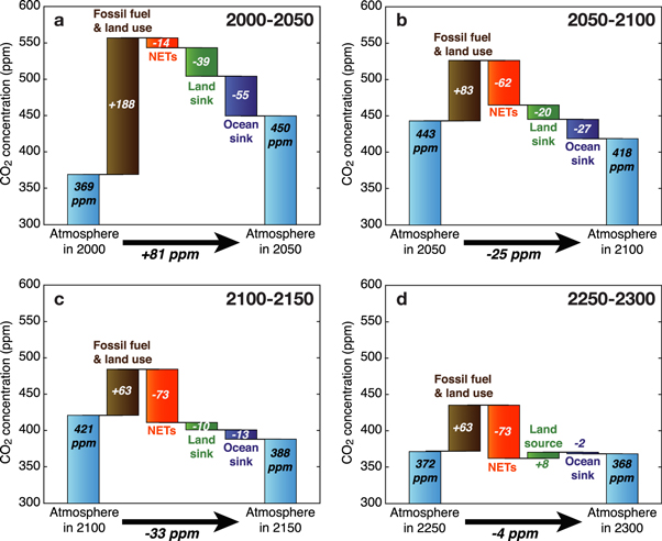
Figure 4. The four stages of succession of the differing balance between flux components. As for figure 1 the bars show changes in atmospheric CO2 (ppm) due to that emission or flux. Each panel shows a selected 50 year period from the RCP2.6 simulations to analyze the changing balance of the flux components. Due to small differences between the compatible emissions diagnosed from the four ESMs and the emissions in the scenario each 50 year period does not balance precisely (see SI for details).
Download figure:
Standard image High-resolution imageIn summary, these results show a clear succession of events: from 2000 to 2050 the emergence of NETs has a slowing effect on anthropogenic emission but the general balance is not changed from the historical period; from 2050 to 2100 natural sinks outweigh (still positive) anthropogenic emissions and CO2 begins to fall; from 2100 to 2250 NETs exceed fossil emissions and human activity is a global negative emission; finally, from 2250 to 2300 natural sinks saturate and reverse and oppose any further removal.
3. State and scenario dependence of the Earth system response
We know that natural carbon sinks and the AF of emissions are sensitive to climate change and behave differently under different future scenarios. It is therefore important to understand how the effectiveness of NETs may also differ depending on the scenario against which they are applied. In this section we look at the range of Earth system responses to different levels of negative emissions when applied under different climate and CO2 scenarios.
To this end we perform new simulations as perturbations to the RCP set of projections. Using the Hadley Centre Simple Climate-Carbon Model widely used in previous studies (Jones et al 2003, 2006, House et al 2008, Huntingford et al 2009—see SI for more details) we quantify the effect of the level of past emissions and climate change on the effectiveness of different levels of NETs.
We take each of the four RCP emissions scenarios as a baseline and apply on top of them four idealised scenarios of additional negative emissions (figure 5(a)). The negative emissions scenarios we impose all begin in 2020 and comprise:
- (a)Constant removal of 1 GtC yr−1.
- (b)Constant removal of 4 GtC yr−1.
- (c)A linear increase in removal from 1 GtC yr−1 in 2020 up to 4 GtC yr−1 in 2080 followed by sustained 4 GtC yr−1 removal until 2100.
- (d)The same as (c) but reversed in time to remove 4 GtC yr−1 from 2020 to 2040 and then gradually reduce the removal rate to 1 GtC yr−1 by 2100.

Figure 5. Simulated CO2 concentration under four RCP emissions scenarios with added idealised profiles of CO2 removal from NETs. The top panels show the inputs to the model: (a) the idealised NET profiles and (b) the total anthropogenic emissions when these NETs are added to the RCP emissions scenarios. RCP emissions (solid lines) with the idealised NETs added (dashed lines). The bottom panel (c) shows the resulting atmospheric CO2 simulated by the simple carbon cycle model.
Download figure:
Standard image High-resolution image
The total CO2 removal for the 2020–2100 period under these idealised scenarios is 80 and 320 GtC under the first two and 230 GtC for the last two. The idealised NET profiles are added to the four RCP emissions scenarios (figure 5(b)). The simple model is run in emissions-driven configuration taking these emissions as input and simulating the response of natural sinks and atmospheric CO2 concentration (figure 5(c)). Here we explore the effect of the applied negative emission and to what extent the Earth-system response depends on the magnitude or time profile of the NET or the state or scenario of background climate and CO2.
Figure 5(c) shows the obvious result that with additional NETs applied to each scenario, the simulated CO2 is reduced. But the degree of reduction varies significantly between scenarios. For example, the same 320 GtC removal results in reduced atmospheric CO2 by 178, 211, 237 and 274 GtC for RCP2.6 to RCP8.5 respectively. It is clear that the effectiveness of negative emissions varies depending on the scenario and the state of the Earth system. It is therefore desirable to define a new metric that can measure this dependence.
The AF is a commonly used metric and we adopt it here to allow a first analysis of the results. It can be defined as an instantaneous value as the ratio of a single year rise in CO2 divided by that year's emissions, or a long-term cumulative quantity defined as the change over many years of CO2 divided by the cumulative emissions over that period. When considering either emissions close to zero or CO2 changes that can change sign, then the former definition is not always well behaved or well defined, and so we adopt the latter definition (hereafter named the cumulative airborne fraction, CAF).
Table 2 shows the cumulative emissions and their impact on atmospheric CO2 for the scenarios with and without added negative emissions over the 80 year period from 2020–2099. The table shows the CAF for the un-modified RCP scenarios, and then also for each modified scenario. A detailed derivation of the terms shown in table 2 is given in the supplementary information.
Table 2. Cumulative emissions and changes in atmospheric CO2 for the simple model simulations of the original and modified RCPs with additional NET scenarios added. The cumulative airborne fraction (CAF) is calculated for the scenarios and also just for the NET components as described in the text.* The definition and calculation of these metrics is explained in more detail in the SI.
| RCP scenario | Idealised NET profile/GtC yr−1 | RCP cumulative emission (2020–2099)/GtC | Cumulative additional NE/GtC | Cumulative total emission (2020–2099)/GtC | Change in atmospheric CO2/GtC | CAF of back-ground RCP* (2020–2099) | CAF of modified RCP * with NET (2020–2099) | Perturbation-AF of the additional negative emission * |
|---|---|---|---|---|---|---|---|---|
| RCP2.6 | 243 | 37 | 0.15 | |||||
| −1 | −80 | 163 | −10 | −0.06 | 0.6 | |||
| −4 | −320 | −77 | −141 | 1.83 | 0.57 | |||
| −1 to −4 | −230 | 13 | −101 | −7.8 | 0.6 | |||
| −4 to −1 | −230 | 13 | −86 | −6.6 | 0.55 | |||
| RCP 4.5 | 663 | 316 | 0.48 | |||||
| −1 | −80 | 583 | 261 | 0.45 | 0.7 | |||
| −4 | −320 | 343 | 105 | 0.3 | 0.67 | |||
| −1 to −4 | −230 | 433 | 155 | 0.35 | 0.7 | |||
| −4 to −1 | −230 | 433 | 169 | 0.39 | 0.66 | |||
| RCP 6.0 | 1060 | 649 | 0.61 | |||||
| −1 | −80 | 980 | 588 | 0.6 | 0.78 | |||
| −4 | −320 | 740 | 412 | 0.55 | 0.75 | |||
| −1 to −4 | −230 | 830 | 470 | 0.56 | 0.78 | |||
| −4 to −1 | −230 | 830 | 483 | 0.58 | 0.74 | |||
| RCP 8.5 | 1764 | 1265 | 0.72 | |||||
| −1 | −80 | 1684 | 1195 | 0.71 | 0.89 | |||
| −4 | −320 | 1444 | 991 | 0.68 | 0.87 | |||
| −1 to −4 | −230 | 1534 | 1061 | 0.69 | 0.89 | |||
| −4 to −1 | −230 | 1534 | 1071 | 0.70 | 0.86 |
The CAF of the original RCP scenarios varies markedly across RCPs, with RCP2.6 having a small fraction of cumulative emissions remaining in the atmosphere for the 2020–2099 period (only 15%) while the other RCPs have a higher fraction of cumulative emissions remaining in the atmosphere, ranging from 48% for RCP4.5 to 72% for RCP8.5 (column 7 in table 2, and see SI text and figure S3). This is consistent with previous studies (Ciais et al 2013, Jones et al 2013). When we look at the CAF under the modified scenarios (column 8) we find two things. For RCP2.6 the values vary hugely between the three additional NET scenarios (figure S3e). This is because either or both the cumulative emissions or the change in atmospheric CO2 are negative and this leads to changes in sign of CAF and values greater than one because the denominator in the definition is small. For RCP6 and RCP8.5 (and to some extent for RCP4.5) we find an opposite result—the CAF is rather insensitive to the CO2 removal and stays close to the value from the un-modified scenario. In either case this metric therefore is not very useful as a measure of either the effect of the negative emission on the Earth system or of the Earth system on the negative emission.
We also calculate the fraction of the CO2 removal which has remained out of the atmosphere—i.e. the AF of the negative emission (final column of table 2; figure S3 panels m–p). For each RCP this metric is rather insensitive to the amount of removal and is different from (and generally bigger than) the CAF of the RCP itself for the same period. This means that the effect of NETs on atmospheric CO2 in the long term is more closely controlled by the background scenario and level of climate change than by the amount of NETs themselves. Comparing the ramped removals with different time profiles of the same cumulative amount we see that the response is not strongly affected by the removal pathway. Tokarska and Zickfeld (2015) also calculated a CAF of their carbon removal and found it to be less dependent on the amount of removal than a CAF based on total emissions. Here we have shown that this property applies across the full range of RCP scenarios. We argue that this perturbation AF (PAF) is therefore a more suitable metric to assess the efficiency of NET than the CAF of the emissions from a single simulation.
This result has several significant implications. Firstly, that it is meaningful to define an AF of a perturbed emission on top of a background scenario in order to measure the effect on atmospheric CO2 of the additional emission or removal. Secondly, this PAF is not the same as the AF of the background scenario itself. Hence, if it is desired to calculate the effect of adding or removing an amount of carbon on top of an existing scenario, then knowing the AF of the scenario does not help—one must calculate the AF of the extra carbon removed instead, i.e. the PAF. Thirdly, though, the PAF from a given scenario is rather insensitive to the magnitude and timing of additional emission. This may be expected when the additional emission is a small fraction of the total emitted carbon for the scenario, but it appears to hold here too even for RCP2.6 when the total carbon removal is bigger than the cumulative emission in the underlying scenario. This means that once a PAF has been calculated relative to a scenario it can be approximately applied to other perturbations about that scenario to estimate their eventual impact.
4. Conclusions
Other studies have outlined various socio-economic costs, biophysical limits and implications of different NETs (Fuss et al 2014, Smith et al 2016, Williamson 2016). Here we have shown how NETs interact with the physical climate-carbon cycle system. Our analysis of the Earth system response to negative emissions has provided new insights and identified future research priorities.
Our results contribute to the need to quantify the interactions between the climate, carbon cycle and anthropogenic NETs in determining future redistribution of carbon between atmosphere, land and ocean reservoirs. By viewing the scenarios and the evolution of carbon sinks and sources in a sequence of phases we have revealed qualitatively different behaviour of the Earth system at different points in time. The combined effect of anthropogenic and natural sources and sinks can change over time, sometimes resulting in positive and sometimes negative changes in atmospheric CO2 concentration. The behavior of atmospheric CO2 is not predictable from the instantaneous anthropogenic emission alone, but requires knowledge of past emissions and Earth system state. For example, CMIP5 simulations following the RCP2.6 pathway to 2300 exhibited periods where atmospheric CO2 decreased despite ongoing net positive emissions from anthropogenic activity. Conversely, later in the scenarios, natural sinks weakened and even reversed, especially on land, and offset the effects of globally negative anthropogenic emissions.
We found significant state-dependence of the Earth system behaviour in response to NETs. Our results showed that the effect of NETs on atmospheric CO2 is more closely controlled by the background scenario and level of climate change than by the amount or timing of NETs themselves. We propose a new metric, the PAF, defined as the ratio of CO2 reduction to the amount of NETs applied. This metric can be used to transfer model results that quantify the effect of NETs under a given scenario to estimate the effect of different levels of NETs against the same scenario.
Simplified climate-carbon cycle models, calibrated against complex ESMs and often used in IAMs for scenario generation are capable of reproducing this behaviour at a global scale. This means that existing IAMs are not systematically wrong in their estimates of NETs required within scenarios. However, large uncertainty remains, due primarily to model spread in the simulation of future carbon sinks and this hinders robust determination of carbon budgets to meet climate targets.
ESMs still lack some important processes such as the role of nutrient cycles that may limit future land carbon storage (Zaehle et al 2015), burning of old land carbon stocks (e.g. peat fires in Indonesia, Lestari et al 2014) or release of carbon from thawing permafrost (Schuur et al 2015). The latter in particular has potentially significant impacts on the requirement for negative emissions, as once released from thawed permafrost it would take centuries to millennia for the same carbon to re-accumulate, making it effectively irreversible on human timescales (MacDougal et al 2015). Uncertainty also exists on the strength and persistence of concentration-dependent carbon uptake, especially on land (so-called 'CO2 fertilisation'). IPCC 5th Assessment Report assessed 'low confidence on the magnitude of future land carbon changes' (Ciais et al 2013). It is increasingly important to bring observational constraints to bear to reduce this uncertainty especially focusing on low emissions scenarios.
It is increasingly clear that negative emissions could be very important in achieving ambitious climate targets, and in fact many scenarios rely on them to do so. Failure to accurately account for carbon cycle feedbacks which increase the need for such negative emissions may strongly and adversely affect the feasibility of achieving these targets. We lack important understanding about the costs and implications of negative emissions, and also knowledge related to the Earth-system dynamics. It is vital to address these knowledge gaps in order to quantify the requirement for, and implications of negative emissions.
Acknowledgments
The work of CDJ, JAL and AW was supported by the Joint UK BEIS/Defra Met Office Hadley Centre Climate Programme (GA01101). CDJ, JAL, AW, PF, EK and DvV are supported by the European Union's Horizon 2020 research and innovation programme under grant agreement No 641816 (CRESCENDO). GPP was supported by the Norwegian Research Council (project 209701). PC acknowledges support from the European Research Council Synergy grant ERC-2013-SyG-610028 IMBALANCE-P. We acknowledge the World Climate Research Programme's Working Group on Coupled Modelling, which is responsible for CMIP, and we thank the climate modeling groups (listed in table 1 of this paper) for producing and making available their model output. For CMIP the US Department of Energy's Program for Climate Model Diagnosis and Intercomparison provides coordinating support and led development of software infrastructure in partnership with the Global Organisation for Earth system Science Portals.