

Abstract
Scientific challenges exist on how to extract information from the wide range of projected impacts simulated by crop models driven by climate ensembles. A stronger focus is required to understand and identify the mechanisms and drivers of projected changes in crop yield. In this study, we investigate the robustness of future projections of five metrics relevant to agriculture stakeholders (accumulated frost days, dry days, growing season length, plant heat stress and start of field operations). We use a large ensemble of climate simulations by the MIT IGSM-CAM integrated assessment model that accounts for the uncertainty associated with different emissions scenarios, climate sensitivities, and representations of natural variability. By the end of the century, the US is projected to experience fewer frosts, a longer growing season, more heat stress and an earlier start of field operations—although the magnitude and even the sign of these changes vary greatly by regions. Projected changes in dry days are shown not to be robust. We highlight the important role of natural variability, in particular for changes in dry days (a precipitation-related index) and heat stress (a threshold index). The wide range of our projections compares well the CMIP5 multi-model ensemble, especially for temperature-related indices. This suggests that using a single climate model that accounts for key sources of uncertainty can provide an efficient and complementary framework to the more common approach of multi-model ensembles. We also show that greenhouse gas mitigation has the potential to significantly reduce adverse effects (heat stress, risks of pest and disease) of climate change on agriculture, while also curtailing potentially beneficial impacts (earlier planting, possibility for multiple cropping). A major benefit of climate mitigation is potentially preventing changes in several indices to emerge from the noise of natural variability, even by 2100. This has major implications considering that any significant climate change impacts on crop yield would result in nation-wide changes in the agriculture sector. Finally, we argue that the analysis of agro-climate indices should more often complement crop model projections, as they can provide valuable information to better understand the drivers of changes in crop yield and production and thus better inform adaptation decisions.
Export citation and abstract BibTeX RIS
1. Introduction
Climate change is expected to have a substantial impact on agricultural production because agriculture is highly dependent on climate variables such as precipitation, temperature, and radiation. The vulnerability of agriculture and food security to climate change has been extensively investigated, generally relying on biophysical models [1–4] or empirical models [5–8]. Such studies, even though they use very different sets of crop models, indicate strong negative impacts of climate change without adaptive measures, but with a large uncertainty in the range of impacts. The wide range of projected impacts on agriculture is driven by both the uncertainty in climate projections and the structural (or parameterization) differences between crop models. While using climate ensembles with crop models is increasingly common to project the potential impacts of climate change on agriculture, scientific challenges exist on how the uncertainty is analyzed and the information is extracted from models that are sometimes used as black boxes [9]. For this reason, a stronger focus is required to understand and identify the mechanisms and drivers of projected changes in crop yield, especially in light of natural variability and potential future changes in extreme events.
Various metrics and indices have also been developed to address the vulnerability of agricultural production under climate change. Many of these indices focus on moisture availability or drought as the most significant climate impact on crop yields. The Palmer drought severity index, standardized precipitation index, NOAA drought index, and Palmer Z-index are widely used [10–12]. New indices, such as the standardized precipitation evapotranspiration index [13], soil moisture deficit index and evapotranspiration deficit index [14], continue to be developed and provide valuable information to farmers [15]. While each of these climate indices provides important insight on agricultural responses under climate change, [10] show that there are significant variations in model performance depending on the choice of drought indices. More recently, studies have focused on agro-climate or agro-meteorological indices that are designed to assess the potential changes in crop exposure to temperature (heat and cold) and water stresses [16–18]. In addition, metrics relevant to management practices, such as start of field operations and growing season length, provide additional value to farmers and decision makers [19]. Therefore, a comprehensive evaluation of both agro-climate and management metrics can help address agriculture vulnerability under climate change.
In this study, we investigate future agro-climate projections using indices shown to be relevant to land management stakeholders, identify the associated impacts on agriculture, and estimate the benefits of greenhouse gas mitigation. Soil water balance metrics are highly relevant to stakeholders and are commonly included in climate change studies, but other metrics are also important and often ignored. We examine the robustness of future projections of these agro-climate indices using a large ensemble of integrated economic and climate projections prepared for the US Environmental Protection Agency's Climate Change Impacts and Risks Analysis (CIRA) project [20]. Using this large ensemble, we investigate the role of multiple sources of uncertainty in global and regional climate projections—including the emissions scenario, the global climate system response (climate sensitivity) and natural variability—on the impact of climate change and greenhouse gas mitigation on agriculture. We further compare our analysis to a multi-model ensemble based on 31 different climate models from the coupled model intercomparison project phase 5 (CMIP5, see [32]). Section 2 describes the agro-climate indices, the climate model and observational data and the methodology used in this study. Section 3 presents the results of the analysis, focusing on the role of uncertainty and the benefits of mitigation. Section 4 provides a summary and discussion, with concluding remarks in section 5.
2. Methodology
2.1. Agro-climate indices
We follow [18] and use five agro-climate indices developed by [19] that were deemed 'very' or 'quite' useful by land management stakeholder focus groups. Not only do these metrics have little conceptual overlap, they also account for various stresses of land productivity and management practices. Table 1 provides a description and methodology for the calculation of these five indices. Accumulated frost days (AFD) serves as a frost index that relates to both cold stress and incidence of pest and disease. Dry days (DD), the number of days with precipitation below a threshold, is used here as a drought index, instead of using more sophisticated indices related to soil moisture that are not necessarily well simulated by climate models [21, 22]. Growing season length (GSL), calculated as the number of days between the last frost (minimum daily temperature below 0 °C) in the spring and the first hard frost in the fall [23, 24], relates to the timing and length of the growing season, which can have far reaching consequences for plant and animal ecosystems [25]. Plant heat stress (PHS), the number of days with daily maximum temperature above a threshold, identifies the risk of heat stress and the associated yield decline. Various thresholds can be used for specific plants or crops; in this study we use a threshold of 29 °C, which corresponds to maize, a major US crop [6], although different thresholds (i.e. 30 °C for soybeans or 32 °C for cotton) do not change the conclusions of the our study. Finally, the start of field operations (SFO), calculated as the date of thermal accumulation of 200 °C, is an index derived from workshops with agricultural stakeholders that refers to the earliest date in a year when a field might be usefully cultivated [19].
Table 1. Selected agro-climate indices, including type, unit, and description of calculation based on [18] and [19], customized for the United States.
| Index | Type | Units | Description |
|---|---|---|---|
| Accumulated frost days (AFD) | Count | Days | Days where Tmin < 0 °C |
| Dry days (DD) | Count | Days | Days when P <1 mm |
| Growing season length (GSL) | Count | Days | Days between the last frost in the spring and the first frost in the fall |
| Plant heat stress (PHS) | Count | Days | Days when Tmax > 29 °C |
| Start of field operations (SFO) | Date | Day of year | Day when the sum of Tavg from 1st January is greater than 200 °C |
Tmin, Tavg and Tmax refer to, respectively, the daily minimum, daily mean and daily maximum temperature at 2 m height (in °C); P refers to daily mean precipitation (in mm).
2.2. Climate model data
We use a 45-member ensemble of simulations using the MIT Integrated Global System Model-Community Atmosphere Model (IGSM-CAM) modeling framework [26] developed for the US Environmental Protection Agency's climate CIRA project [20]. This ensemble is made up of three consistent socioeconomic and emissions scenarios: a reference scenario (REF) with unconstrained emissions and two greenhouse gas mitigation scenarios that rely on a uniform global carbon tax to stabilize radiative forcing at 4.5 W m−2 (POL4.5) and 3.7 W m−2 (POL3.7) by 2100. More details on the emissions scenarios and economic implications, along with how they relate to the representative concentration pathway (RCP) scenarios [27], are given in [28]. For each emissions scenario, the IGSM-CAM was run with three values of climate sensitivity (CS = 2.0°, 3.0° and 4.5 °C), corresponding to the likely range and best guess, obtained via radiative cloud adjustment (see [29]). For each climate sensitivity, a five-member ensemble was run to produce different representations of natural variability, thus resulting in a 15-member ensemble for each emissions scenario. A detailed procedure for the design of the large IGSM-CAM ensemble used in this study, along with an analysis of the climate projections for the US, can be found in [30]. Because we use integrated economic and climate projections obtained using an Integrated Assessment Model (IAM), we can directly attribute the differences in future agro-climate projections between the different emissions scenarios to explicit policy choices, thus identifying the benefits of greenhouse gas mitigation. Furthermore, while this ensemble is derived using a single climate model, it accounts for the uncertainty in emissions scenarios, global climate response and natural variability, which accounts for a substantial share of the full uncertainty in future climate projections [30]. We analyze 20-year time periods over five different representations of natural variability, resulting in 100 years to define changes in 2050 (defined as the period 2041–2060) and 2100 (defined as the period 2081–2100) relative to present day (defined as the period 1991–2010), in order to obtain robust estimates of the anthropogenic signal and thus identify the benefits of greenhouse gas mitigation. We also identify the various uncertainties represented in the modeling framework.
To provide some context to the agro-climate projections using the IGSM-CAM ensemble, we compare our results to the CMIP5 multi-model ensemble under the RCP8.5 and RCP4.5 scenarios. We compute the agro-climate indices using historical and future simulations from 31 climate models (see the supplemental materials for a complete list) after interpolating the required input data to the same 2° × 2.5° grid as the IGSM-CAM. The 31 models considered were those for which the required daily inputs for both emissions scenarios were available at the time of the study. Only one run is used for each model, even when an ensemble (i.e. with different initial conditions) was run.
2.3. Observational data
We evaluate the capability of the IGSM-CAM to simulate the five agro-climate indices for present-day conditions using two independent observational datasets: the National Aeronautics and Space Administration Modern Era Retrospective-Analysis for Research and Applications (MERRA) reanalysis [33], at 0.5° × 0.66° resolution, and the National Centers for Environmental Prediction/National Center for Atmospheric Research (NCEP/NCAR) Reanalysis [34], at T62 gaussian grid (approximately 2° × 2° resolution). We rely on two different reanalysis datasets to illustrate—not quantify, as this would require a more complete analysis—the uncertainty in observational datasets that include the role of lower resolution that climate models suffer from.
2.4. Time of emergence
We investigate the robustness of the agro-climate projections by estimating when the signal (S) of anthropogenic changes is emerging against the noise (N) of natural variability. There is no single metric of emergence and various studies have used different definitions of S and N to estimate the signal-to-noise ratio (S/N). For example, [35] define the warming signal by regressing temperature at each grid cell of a climate model simulation against a smoothed version of its global mean temperature, and they define the noise as the interannual standard deviation from a pre-industrial control simulation. In [36], the authors define the signal as a 10 year mean anomaly and the noise as the interannual standard deviation from a transient historical simulation. Meanwhile, [37] define the signal of precipitation change as the 20 year mean anomaly of a multi-model ensemble mean and the noise as intermodel spread and internal multi-decadal variability. Finally, [38] analyzes the time of emergence of seasonal temperature changes using a large ensemble of climate simulations with different initial conditions, where the signal is the ensemble mean and the noise the standard deviation of internal variability computed for each year across the ensemble (after a 10-year running mean). In this study, we estimate the signal (S) for each agro-climate index as the 20 year running mean anomaly from present day for each climate simulation and the noise (N) as the interannual standard deviation from a pre-industrial control simulation. We then define the time of emergence as the first year in which the S/N exceeds a threshold of 2.
3. Results
Figure 1 shows the evaluation of the IGSM-CAM simulation of the five agro-climate indices for present-day conditions compared to the two reanalysis datasets. Overall, the MIT IGSM-CAM exhibits a very good capability to reproduce the magnitude and spatial features of the agro-climate indices. The two reanalysis products show a good agreement with each other in both the magnitude and spatial distribution of the indices. Nonetheless, noticeable inconsistencies exist that can be attributed to differences in observational datasets assimilated in the climate models, differences between the climate models used (including resolution), and the methodology for data assimilation. Generally, the IGSM-CAM bias falls within the range of the two observation datasets and is largely driven by the lower resolution of the climate model. The AFD and SFO indices show a strong north–south gradient, with largest values over the Rocky Mountains, the Great Lakes and New England. The GSL and PHS show the opposite pattern, with the largest values in the South. The strongest DD values are over southwestern states and the Great Plains. As expected from any climate model, systematic biases are present and consistent with previous evaluations of the model [26, 31]: the IGSM-CAM exhibits a warm bias in the Midwest and a dry bias in the Southeast. This warm bias can be identified in the AFD and PHS indices, and to a lesser extent in the GSL and SFO indices while the dry bias is associated with a positive bias in the DD index. Altogether, the IGSM-CAM shows reasonable skills at reproducing the major characteristics of the agro-climate indices over the US.
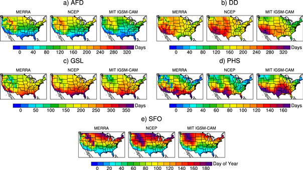
Figure 1. US maps of present-day (1991–2010) (a) accumulated frost days (AFD), (b) dry days (DD), (c) growing season length (GSL), (d) plant heat stress (PHS) and (e) start of field operations (SFO) for the MERRA reanalysis, NCEP Reanalysis and simulated by the MIT IGSM-CAM. The mean over the five members with different representations of natural variability for CS = 3.0 °C is shown for the MIT IGSM-CAM.
Download figure:
Standard image High-resolution imageFigure 2 shows maps of forced changes in each agro-climate index in 2100 relative to present day, for each climate sensitivity considered (CS = 2.0°, 3.0° and 4.5 °C) and for the REF and POL4.5 scenarios. For each emissions scenario and climate sensitivity, the forced changes are estimated as the mean over the five-member ensemble with different representations of natural variability, thus producing a 100-year mean (20-year period window, five simulations). The IGSM-CAM simulates a very wide range of changes in agro-climate projections, from little change under the POL4.5 scenario for the low climate sensitivity to very large changes under the REF scenarios for the high climate sensitivity. The greenhouse gas mitigation significantly reduces the projected changes, even when considering the uncertainty in the global climate system response represented by the climate sensitivity: the projected changes under the POL4.5 scenario with the high climate sensitivity (CS = 4.5 °C) is always lower than the projected changes under the REF scenario with the low climate sensitivity (CS = 2.0 °C). In addition, the patterns of change are similar for each climate scenario (climate sensitivity and emissions scenario), largely because of the use of a single model and the large averaging period used (100 years). The AFD index is projected to decrease the most in the Rocky Mountains, the Great Lakes and New England (around 60–100 days under REF, half under POL4.5). A similar pattern can be seen for the SFO, which projects to start earlier (negative values) especially in these regions, by as much as 75–100 days under REF and half under POL4.5. Increases in the GSL are largest over the Northwest and the NorthEast (from 70 to 100 days under REF, from 15 to 50 days under POL4.5). PHS is projected to increase the most over the western US, the Gulf Coast and the East Coast (from 40 to 80 days under REF, 10–30 days under POL4.5). Finally, DD are projected to increase in the western US (as much as 30 days under REF, half under POL4.5) and decrease elsewhere (30–40 days under REF, half under POL4.5), especially over the Great Plains. This dipole pattern is consistent with the tendency of the IGSM-CAM, as well as the Community Climate System Model version 3, which shares the same atmospheric component (CAM).
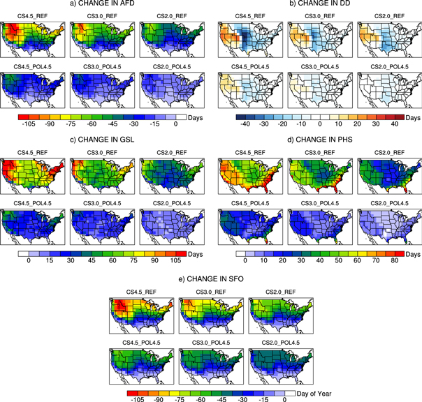
Figure 2. US maps of projected forced changes in (a) accumulated frost days (AFD), (b) dry days (DD), (c) growing season length (GSL), (d) plant heat stress (PHS) and (e) start of field operations (SFO) in 2100 (2081–2100) relative to present day (1991–2010), simulated by the MIT IGSM-CAM for each climate sensitivity considered (CS = 2.0°, 3.0° and 4.5 °C) and for the REF scenario (top panel) and the POL4.5 scenario (bottom panel). For each emissions scenario and climate sensitivity, the forced changes are estimated as the mean over the five-member ensemble with different representations of natural variability.
Download figure:
Standard image High-resolution imageFigure 3 shows maps of changes in each agro-climate index in 2100 relative to present day, for each ensemble member with different representations of natural variability for the simulations with a climate sensitivity of 3.0 °C under the POL4.5 scenario. This analysis identifies the uncertainty in natural variability—in particular multi-decadal variability—since the maps show 20-year mean changes. The impact of natural variability varies greatly by index. For changes in AFD and in SFO, different representations of natural variability mainly affect the magnitudes of the projected changes, but not the patterns of change. On the other hand, changes in the other three indices present different magnitudes and patterns, and even different signs. This is particularly striking given the long period of averaging. While all members show a general tendency for increases in DD in the West (and decreases elsewhere), different members exhibit different magnitudes and extents of change. For example, member 2 projects a weak decrease in DD in the central US but a clear increase in the West, and member 3 displays a clear decrease over most of the US with only a little increase on the West Coast. This implies less robustness in the projections of changes in DD compared to changes in AFD and SFO. This is consistent with previous findings on the large uncertainty associated with natural variability for precipitation changes [31, 39, 40]. The GSL and PHS are also clearly impacted by the role of natural variability. While all members show patterns generally consistent with the ensemble mean shown in figure 2—for GSL, the largest increases in the Northwest and the smallest increases in the South; for PHS, the largest increases in the western US, the Gulf Coast and the East Coast—individual members disagree on the magnitude and spatial extent of the largest changes, and can even disagree on the sign in specific regions. For example, member 3 projects widespread decreases in PHS over major parts of the Great Plains and some decreases in GSL over a small part of Texas. This implies little robustness in the projections of changes in GSL and PHS in these regions, which is surprising given the general assumption of robustness in temperature-related simulations. The same analysis for the REF scenario in 2050 and in 2100 is shown in the supplemental materials. It reveals that the relative role of natural variability is lessened under a scenario with a larger forcing. At the same time, the absolute range associated with natural variability remains constant among scenarios and time periods, corresponding to the irreducible error in the projections, as shown in [30].

Figure 3. US maps of projected changes in (a) accumulated frost days (AFD), (b) dry days (DD), (c) growing season length (GSL), (d) plant heat stress (PHS) and (e) start of field operations (SFO) in 2100 (2081–2100) relative to present day (1991–2010), simulated by the MIT IGSM-CAM for each member with different representations of natural variability for CS = 3.0 °C and POL4.5 scenario.
Download figure:
Standard image High-resolution imageFigure 4 shows a summarized analysis of the range of projected changes in each agro-climate index, area-averaged over the US, in 2050 and 2100 relative to present day. The range is estimated over the 15-member IGSM-CAM ensemble with different climate sensitivities and representations of natural variability for each emissions scenarios and over the CMIP5 multi-model ensemble (31 models) under the RCP8.5 and RCP4.5. We also show the 1 and 2 standard deviation of the natural variability derived from a pre-industrial control simulation of the IGSM-CAM to provide a brief signal-to-noise analysis. The US as a whole is projected to experience fewer frosts, a longer GSL, an earlier SFO, an increase in heat stress. The range of changes is particularly wide under the REF scenario, especially by 2100, with the upper bounds close to twice as large as the lower bound. For example, increases in GSL under REF by 2100 range from 38 to 82 days, and decreases in AFD range from 32 to 60 days. The implementation of either greenhouse gas mitigation scenario considered in this study cuts by half most of the changes projected under the unconstrained scenario. In addition, the range of changes for the unconstrained and mitigation scenarios do not overlap, thus indicating robust benefits of mitigation. At the same time, there is little difference between the two mitigation scenarios, given the overall uncertainty. Finally, the lack of robustness in the projections of changes in DD, eluded earlier, are further substantiated by this analysis, as they are within the noise from natural variability even by 2100. The comparison between the IGSM-CAM ensemble and the CMIP5 ensemble reveals similar changes in temperature-related indices. While the exact magnitude of the changes is not in precise agreement, the range is in agreement. Since the RCP scenarios and the CIRA scenarios were designed independently, a simple metric like the radiative forcing in 2100 is not sufficient to expect perfect agreement. For the DD index, both ensembles project a range of changes that span both increases and decreases, but the CMIP5 range is wider. In addition, the CMIP5 ensemble projects a mean increase in DD while the IGSM-CAM mean is negative. At the same time, the statistical significance of these changes is likely to be weak since they fall within the noise of natural variability.
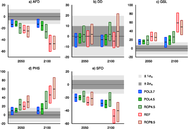
Figure 4. Projected changes in (a) accumulated frost days (AFD), (b) dry days (DD), (c) growing season length (GSL), (d) plant heat stress (PHS) and (e) start of field operations (SFO), area-averaged over the US, in 2050 (2041–2060) and 2100 (2081–2100) relative to present day (1991–2010) simulated by the MIT IGSM-CAM for all three emissions scenarios (REF, POL4.5 and POL3.7) and by 31 CMIP5 models for the RCP4.5 and RCP8.5 scenarios. Box plots show the range over the 15-member IGSM-CAM ensemble with different climate sensitivities and representations of natural variability for each emissions scenario and over the CMIP5 multi-model ensemble (31 models) under the RCP8.5 and RCP4.5. The black horizontal lines show the mean of the IGSM-CAM simulations for the medium climate sensitivity (CS = 3.0 °C) for each emissions scenario and the mean over the 31 CMIP5 models for the RCP8.5 and RCP4.5. Dark (light) gray shading represent the 1 (2) standard deviation of the natural variability estimated from a pre-industrial control simulation with the IGSM-CAM.
Download figure:
Standard image High-resolution imageWe explore in more detail the S/N by estimating the time of emergence, in each simulation, of the US mean changes in the five agro-climate indices, and computing the range for each emissions scenario (see figure 5). This analysis reveals a large uncertainty in the estimates of the time of emergence, indicating very different behaviors between indices and scenarios. Changes in DD do not emerge from the noise before 2100 for all three scenarios, confirming the lack of robustness in projections of precipitation changes. At the same time, the time of emergence of changes in SFO occurs between 2025 and 2050 in all the simulations, implying little impact of the mitigation scenarios. For all other indices, the benefits of mitigation are clear. Under REF, changes emerge from the noise by 2070 at the latest (and as early as 2020). The implementation of either mitigation scenarios allows for the possibility that the projected changes remain within the noise of natural variability by 2100. That is generally the case for simulations with the lower climate sensitivity (CS = 2.0 °C), which illustrates the need to account for the uncertainty in the global climate system response in analysis of the benefits of climate mitigation. Finally, the difference between the two policy scenarios is generally small. It is only noticeable for projections of changes in PHS—by reducing the probability of emergence before 2100—and for changes in AFD—by increasing the mean estimate of the time of emergence, but not its range.

Figure 5. Time of emergence of the projected US mean changes relative to present day (1991–2010) in accumulated frost days (AFD), dry days (DD), growing season length (GSL), plant heat stress (PHS) and start of field operations (SFO) simulated by the MIT IGSM-CAM for all three emissions scenarios (REF, POL4.5 and POL3.7). Box plots show the range over the 15-member IGSM-CAM ensemble with different climate sensitivities and representations of natural variability for each emissions scenario. The vertical black lines show the mean of the IGSM-CAM simulations for the medium climate sensitivity (CS = 3.0 °C) for each emissions scenario. The time of emergence is shown for a signal-to-noise ratio (S/N) greater than 2. Dotted lines past 2100 indicate that the signal has not emerged from the noise by 2100.
Download figure:
Standard image High-resolution image
4. Summary and discussion
Under climate change, this study generally projects the US as a whole to experience fewer frosts, a longer GSL, an earlier SFO, an increase in heat stress and no robust changes in DD. However, these changes have specific regional patterns. The northern US, especially over the Rocky Mountains, the Great Lakes region and New England project to benefit from less cold damage and earlier planting, ensuring maturation and the possibility for multiple cropping—although fewer frosts could also lead to higher risks of pest and disease. The southern US is expected to suffer from a stronger heat stress without the associated benefit of a significant increase in the GSL. This north–south disparity in agro-climate projections is consistent with the changes in yield projected by [8]. The West is shown to experience more heat stress and more DD, which could result in declining yields and negative implications for water resources and irrigated agriculture.
These projections are associated with large uncertainties in magnitude, spatial pattern and even sign. This study finds that the magnitude of the changes is largely controlled by the climate sensitivity and emissions scenario. Meanwhile, natural variability can cause large differences in the regional patterns of the projected changes—especially for changes in DD, GSL and PHS—including reversals of the sign of the projected changes locally. That is true even using a 20 year averaging period, indicating that future changes in agro-climate indices are not always predictable locally. This study further highlights the lack of robustness of projected changes in precipitation, as demonstrated by the lack of emergence of US mean changes in DD from the noise of natural variability, even by 2100. Our findings suggest that changes in temperature-related agro-climate indices are generally more predictable than metrics based on precipitation. The substantial role of natural variability on future climate projections has gained a great deal of interest over the past few years [30, 31, 39, 41–44], and we hope this study sheds some light on the implications for projections of future climate change impacts on US agriculture. In particular, we caution policymakers and land management stakeholders to properly examine the robustness of agro-climate projections when developing and evaluating strategies to adapt agriculture to climate change.
A comparison of the IGSM-CAM ensemble to the CMIP5 multi-model ensemble provides further insight into the uncertainty in agro-climate projections over the US. We find that a single climate model, with different emissions scenarios, climate sensitivities and representations of natural variability, simulates a range of changes similar to 31 different climate models. Our analysis suggest that multi-model uncertainty can be largely be explained by differences in the climate sensitivity of the models and differences in initialization that leads to different representations of natural variability in the different simulations. This finding is particularly true for temperature-related indices, but less so for projections of precipitation changes, which are less robust to start with. While the IGSM-CAM projects both increases and decreases in DD, it does not reproduce the wide range of changes simulated by the CMIP5 ensemble. Nonetheless, we argue that sampling key sources of uncertainty in a single climate model provides a complementary framework to the commonly used multi-model ensemble. In addition, using an IAM to derive integrated economic and climate projections provides a major advantage, i.e. differences between scenarios can be attributed to an explicit choice of climate policy and the benefits of greenhouse gas mitigation can be directly estimated (see [28, 45]). In contrast, because the underlying socio-economic trajectories and priorities are not consistent in the RCP scenarios, differences between the scenarios cannot be attributed to policy choices. Meanwhile, our framework even allows us to compare two greenhouse mitigation scenarios that only differ by the stringency of the carbon tax applied.
The analysis shows that the projected changes in the five agro-climate indices are significantly reduced under the two policy scenarios compared to the reference scenario, especially by 2100. On average, the implementation of either greenhouse gas mitigation scenario cuts by half the changes projected under the unconstrained scenario. As a result, greenhouse gas mitigation has the potential to significantly reduce adverse effects of climate change (i.e. higher heat stress, higher risks of pest and disease from fewer frost days), while also curtailing potentially beneficial impacts (i.e. earlier planting, a longer growing season with possibility for multiple cropping, and less frost damage). We also find that climate mitigation can potentially prevent changes in several indices to emerge from the noise of natural variability, even by 2100. This is likely to be a major benefit from mitigation given that any significant climate change impacts on crop yield, whether beneficial or damaging, will result in nation-wide changes in the agriculture sector. The cost of adaptation at that scale, such as the northward displacement of crop production, is difficult to quantify. Finally, we find that differences between the two mitigation scenarios are difficult to distinguish and that the benefits of mitigation are present in 2050, but small. The benefits of climate mitigation on projections of future changes in agro-climate indices resonates with prior studies using crop models [3, 8]. At the same time, we realize that increases in CO2 concentrations and adaptive management can provide significant mitigation of the negative effects of climate change [46–48].
5. Conclusion
This study shows that projections of agro-climate indices that are relevant to stakeholders can provide great insight into the fate of future climate change impacts on agriculture. While these projections are subject to substantial uncertainty, we show that using a single climate model that accounts for key sources of uncertainty (i.e. emissions scenario, global climate system response, natural variability) provides an efficient and complementary framework to the more common approach of multi-model ensemble (i.e. CMIP5 ensemble). We highlight the important role of natural variability, especially for projections of changes in DD and heat stress, leading to uncertainty in the magnitude and location of the largest changes or even the sign of the projected changes. For this reason, studies of climate change impacts on agriculture must consider these uncertainties by relying on large ensembles of climate projections that sample the major sources of uncertainty—especially natural variability. In addition, using integrated economic and climate projections, we can directly estimate the benefit of climate mitigation. We find that climate mitigation has substantial benefits: it cuts in half the changes projected under an unconstrained scenario, and it potentially prevents changes from emerging from the noise of natural variability. Finally, we argue that agro-climate indices, in combination with crop model projections, can provide valuable information to better understand the drivers of changes in crop yield and production, thus better informing adaptation decisions.
Acknowledgments
This work was partially funded by the US Environmental Protection Agency's Climate Change Division, under Cooperative Agreement #XA-83600001, by the US Department of Energy, Office of Biological and Environmental Research, under grant DE-FG02-94ER61937, and by the National Science Foundation Macrosystems Biology Program Grant #EF1137306. The Joint Program on the Science and Policy of Global Change is funded by a number of federal agencies and a consortium of 40 industrial and foundation sponsors. (For the complete list see http://globalchange.mit.edu/sponsors/current.html). This research used the Evergreen computing cluster at the Pacific Northwest National Laboratory. Evergreen is supported by the Office of Science of the US Department of Energy under Contract No. DE-AC05-76RL01830.