

Abstract
Cannabis agriculture is a multi-billion dollar industry in the United States that is changing rapidly with policy liberalization. Anecdotal observations fuel speculation about associated environmental impacts, and there is an urgent need for systematic empirical research. An example from Humboldt County California, a principal cannabis-producing region, involved digitizing 4428 grow sites in 60 watersheds with Google Earth imagery. Grows were clustered, suggesting disproportionate impacts in ecologically important locales. Sixty-eight percent of grows were >500 m from developed roads, suggesting risk of landscape fragmentation. Twenty-two percent were on steep slopes, suggesting risk of erosion, sedimentation, and landslides. Five percent were <100 m from threatened fish habitat, and the estimated 297 954 plants would consume an estimated 700 000 m3 of water, suggesting risk of stream impacts. The extent and magnitude of cannabis agriculture documented in our study demands that it be regulated and researched on par with conventional agriculture.
Export citation and abstract BibTeX RIS

Original content from this work may be used under the terms of the Creative Commons Attribution 3.0 licence. Any further distribution of this work must maintain attribution to the author(s) and the title of the work, journal citation and DOI.
Introduction
Illegal drug production and distribution are multi-billion-dollar global industries (UNODC 2014) with potential to transform ecosystems (Benessaiah and Sayles 2014, Mcsweeney et al 2014). Drug supply chains are generally thought to involve production in the Global South to satisfy demand in the Global North, but this assumption no longer holds true for cannabis (Cannabis sativa or C. indica) (Decorte et al 2011). The geography of cannabis agriculture is shifting, with import substitution now observed in almost every developed country in the world (Potter et al 2011).
In the United States of America (USA) cannabis agriculture has been understudied and underestimated in scope and magnitude (Weisheit 2011). Research on cannabis agriculture systems is especially urgent in light of recent policy liberalization (Crick et al 2013), which is facilitating a transition in cannabis from an illegal drug to a licit agricultural crop. Cannabis is still federally illegal in the United States as a Schedule 1 drug according to the Drug Enforcement Agency (http://dea.gov/druginfo/ds.shtml), and this classification has stymied research on cannabis production methods and their environmental impacts (Eisenstein 2015). However, over the last two decades the majority of states have liberalized cannabis policy (Cole 2013), ranging from decriminalization to medical permitting to the creation of retail markets for recreational use. The latest federal spending bill prohibits federal agents from interfering with the enactment of state laws allowing medical cannabis use. States are likewise left to address any collateral impacts of the burgeoning medical cannabis industry. State-level regulations have at times included explicit environmental protections, such as laws approved in late 2015 in California meant to hold cannabis agriculture to the same standards as other crops (State of California 2015). In general, policymakers are challenged to keep up with the rapid changes in cannabis agriculture on the ground.
Legal US markets for cannabis were estimated to be worth $2.7 billion in 2014 and projected to reach $11 billion by 2019 (Arcview Market Research 2014). This expanding market, coupled with new opportunities to grow cannabis free from threat of federal enforcement, suggest significant near-term shifts in production. Even with new regulatory protections for the environment and their embrace by many growers (McGreevy 2015), a boom in cannabis agriculture promises serious environmental implications (Carah et al 2015).
Building on other scholars' (Carah et al 2015, Eisenstein 2015, Sides 2015) recognition of cannabis production as a topic of growing environmental concern and their calls for more rigorous research, we present here a study on the expansion and intensification of land use for cannabis agriculture. Our study, as an example of what could be done anywhere cannabis agriculture takes place, illustrates the value of a systematic environmental research approach.
In the current era of policy liberalization, the seat of cannabis agriculture in the United States is a region known as the 'Emerald Triangle' in northern California (Corva 2014). Consisting of Humboldt, Trinity, and Mendocino Counties, the Emerald Triangle is arguably the birth place of modern cannabis production in the US, and Humboldt County might be the top cannabis-producing region in the world (Corva 2014). The Emerald Triangle is also home to outstanding natural resources including large stands of old-growth California redwood (Sequoia sempervirens) and relatively uninterrupted runs of endangered and threatened anadromous fish, such as steelhead trout (Oncorhynchus mykiss) and Chinook salmon (Oncorhynchus tshawytscha). The potential conflict between the rapidly growing cannabis industry and the habitat needed by these protected species is thus a federal-level, as well as a local-level, environmental concern.
Popular media speculation about environmental impacts of cannabis agriculture in this region, especially impacts on water, is widespread (Bland 2014, Harkinson 2014, Ryzik 2014), but empirical research is limited (Carah et al 2015). The small body scientific research points to profound negative consequences, including decreased stream flows (Bauer et al 2015), rodenticide poisoning of rare carnivores (Gabriel et al 2012), and high carbon emissions from greenhouses (Mills 2012). While these studies show negative impacts of cannabis production, they are all based on limited, non-random sampling in areas where cannabis production is known to be high. Thus, they cannot be used to infer impacts at broader scales.
In order to identify the extent of land-use change for cannabis production and other potential impacts on the environment, we systematically mapped grow sites in a random sample of 60 watersheds within and bordering Humboldt County that statistically represent the County a whole. (See supporting online information for sampling details.) We used our map results to answer four questions about cannabis agriculture and its potential impacts on the environment:
- (1)How many cannabis grows are in the study area, and what are the attributes of these grows?
- (2)Are there statistically significant spatial patterns of cannabis production within and across watersheds?
- (3)Do grows threaten natural areas by being located on sensitive sites far from developed infrastructure?
- (4)Do grows pose a risk to threatened species due to their water consumption and location near critical habitat?
Methods
Study area
Our study area consisted of 60 randomly sampled (out of 112 total), ecologically representative watersheds (table SI 1) within and bordering Humboldt County (12 digit WBD) (USGS 2015) (figure 1). The area is characterized physically by steep terrain (34% of land with slope >30°), large areas of forest, and >160 km of Pacific Ocean coastline. Coastal areas are consistently cool with summer high temperatures seldom exceeding 26 °C. By contrast, inland valleys and uplands are warmer in summer and cooler in winter (California 2015).

Figure 1. Sampled watersheds within and adjacent to Humboldt County, California.
Download figure:
Standard image High-resolution imageExcluding cannabis, agricultural sales in Humboldt County totaled nearly $270 million in 2013. Livestock production contributed $76 million, followed by timber ($72 million) milk and dairy products ($61 million), nursery stock ($49 million), field crops ($5 million), and fruit, nut and vegetable crops ($3 million) (Humboldt County 2015). Over 50 000 ha of land is in organic production. Humboldt County participates in the Williamson Act, which reduces property taxes for owners who commit their land to agricultural uses. In forested areas with high timber value, Timber Production Zone designations reduce property tax in exchange for limiting land development potential. Humboldt County producers have access to state, regional and international markets for their products.
Methods of cannabis production are not well known to researchers due to the traditionally illicit nature of the product. Since the prohibition of cannabis in the 1930s, research into horticultural and agronomic methods has been prohibited in the US. Thus, there is no published literature on the modes of production used in our study area. Popular accounts point to three main cannabis production modes in our area: indoor cultivation with artificial light, greenhouse cultivation where light may be natural, artificial, or both, and outdoor cultivation with natural light. Growers report the importation of enhanced soils to make up for poor-quality natural soils throughout the county. There is no research documentation of fertilizer or pesticide use in cannabis production in our area, though both are reported to be used elsewhere (Carah et al 2015).
Data
We located and mapped greenhouse and outdoor grow sites with high-spatial-resolution satellite imagery in Google Earth. The fine spatial grain of this imagery allowed us to visually detect even small, sparsely planted grows, which are not easily captured using spectral remote sensing (Daughtry and Walthall 1998, Kalacska and Bouchard 2011). These grows make up a large proportion of the cannabis agriculture operations in our study area.
Data on critical steelhead trout (Oncorhynchus mykiss) and Chinook salmon (Oncorhynchus tshawytscha) habitat locations were provided by the California Department of Fish and Wildlife (2015). In our study area, these salmonids are listed as threatened under the federal Endangered Species Act (National Oceanic and Atmospheric Administration 2015). We chose to feature these species because they are vulnerable to low flows (imposed by water withdrawals), soil erosion, and agrochemical contamination.
Data on slope and zoning were developed and provided by Humboldt County (http://humboldtgov.org/1357/Web-GIS). We used the Watershed Boundaries Dataset at the Hydrological Unit Code 12 level (USGS 2015). The LANDFIRE dataset was used to determine land cover type (USDA 2013).
Identifying and delineating grow sites
Outdoor grows and greenhouses can be visually detected in high-spatial-resolution satellite imagery (figure 2) (Bauer et al 2015). We used fall images from 2012 and 2013, because cannabis plants are mature at this time and can be distinguished from other vegetation based on their size, arrangement, and color. We demarcated grows using heads-up digitizing within a systematic grid pattern overlaid on each watershed (see SI). For outdoor grows, we counted the number of plants. To estimate plants in greenhouses, we followed Bauer et al (2015) in assuming one plant needs 1.115 m2 of greenhouse area. We assumed all greenhouses are used for cannabis production based on a 19-fold increase in greenhouses 2004–2014, and a simultaneous decrease in nursery crop production (Humboldt County 2015). Checks for data robustness and methods reliability, as well as full mapping procedures are provided in the SI.

Figure 2. Image from Google Earth showing cannabis plants and greenhouse from 2012.
Download figure:
Standard image High-resolution imageSpatial distribution and clustering of grows
We analyzed the distribution and clustering of grow sites (outdoor and greenhouse grows combined) at two scales, within and across watersheds. Across watersheds we calculated a global Moran's I statistic to test for spatial autocorrelation among watersheds with respect to plant density (# of plants/watershed area). We then carried out an optimized hotspot analysis to calculate Getis-Ord Gi* statistics for the study area and for each individual watershed (Getis and Ord 2010). At least 30 grows had to be present in a watershed to calculate the Getis-Ord Gi* statistic, and 26 of 60 watersheds met this standard. The ArcGIS Optimized Hotspot Analysis Tool and Global Moran's I tools were used for these analyses (ESRI 2015).
Threats due to remote and steep grow sites
We overlaid ancillary spatial data in a GIS to derive proxies for potential threats to natural areas. First we calculated the distance from each grow to the nearest developed road as a proxy for fragmentation caused by land clearing and road building. Next we overlaid grows on a >30% slope layer as an indicator of potential for erosion, sedimentation, and mass wasting (landslides, etc).
Potential impacts on threatened freshwater species
To better understand potential impacts on threatened species we calculated the number of plants and grows located within buffers around critical habitat of Chinook salmon and steelhead trout. We complemented our spatial analysis with total water use estimates. To quantify water use in our study, we applied published water use rates per plant (Bauer et al 2015) to the number of plants identified in our mapping exercise. We thus assumed 22.7 liters per plant per day over a 150 day growing season (Humboldt Growers Association 2010).
Results
Number and extent of grows
We located 4428 grow sites in our study area containing an estimated 297 954 plants. The average grow contained 67 (SD 75) plants. Greenhouse grows (n = 2407) contained more plants on average (85.77, SD 88.81) than outdoor grows (n = 2021) (45.23, SD 45.266). The largest outdoor grow had 757 plants, while the largest greenhouse grow had an estimated 960 plants. An average watershed in our study area would contain 70 grows (SD 102) and 4770 plants (SD 6448). The maximum number of grows in one watershed was 481, and the maximum number of plants in one watershed was 26 677. We identified zero grows in 11 watersheds (table 1, figure 3).
Table 1. Summary statistics for individual grows and watersheds.
| Outdoor grows | ||||
|---|---|---|---|---|
| Mean | Std. dev | Min | Max | |
| # Plants | 45.26 | 45.38 | 2 | 757 |
| Water use (m3) | 104.56 | 104.83 | 4.620 | 1748.670 |
| Greenhouse grows | ||||
| Mean | Std. dev | Min | Max | |
| # Plants | 85.77 | 88.81 | 1 | 960 |
| Water use (m3) | 198.15 | 205.16 | 2.31 | 2217.60 |
| All grows | ||||
| Mean | Std. dev | Min | Max | |
| # Plants | 67.28 | 75.06 | 1 | 960 |
| Water use (m3) | 155.43 | 173.39 | 2.31 | 2217.60 |
| Summarized at watershed scale | ||||
| Mean | Std. dev | Min | Max | |
| # Grows | 71 | 102 | 0 | 481 |
| # Plants | 4770 | 6448 | 0 | 26677 |
| Water use (m3) | 11000 | 14900 | 0 | 61600 |
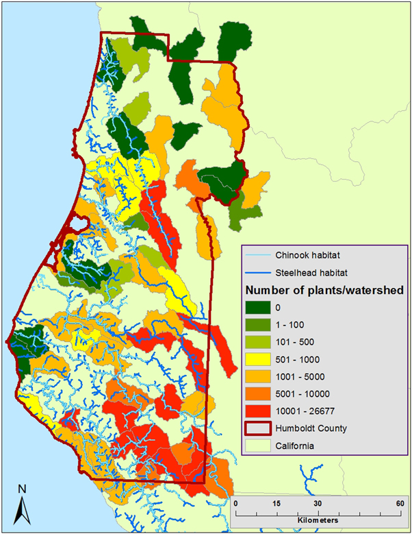
Figure 3. Number of plants per watershed and location of critical habitat for steelhead trout and Chinook salmon.
Download figure:
Standard image High-resolution imageSpatial distribution and clustering of grows
We discovered strong spatial clustering across watersheds in our study area and within watersheds. At the scale of the study area, there is statistically significant positive spatial autocorrelation among watersheds with respect to the density of plants (# of plants/watershed area). The Moran's I was 0.371 (z-score 4.194, p-value 0.000 027). The optimized hot spot analysis applied to the full study area resulted in the identification of three hotspots and one cold spot (figure 4). The optimized hot spot analysis conducted at the individual watershed scale also showed strong clustering, with hot spots present in all 26 watersheds analyzed.
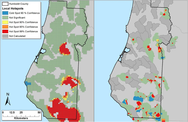
Figure 4. Hot spots of cannabis cultivation in Humboldt County. (A) Results of the optimized hotspot analysis for the whole county. (B) Result of the optimized hotspot analysis run individually for 26 watersheds.
Download figure:
Standard image High-resolution imageProxies for habitat threats
Over 68% of grows were located more than 500 m from a developed road (figure 5(C)), while 15% were within 100 m. Total cultivated area covered by greenhouses and outdoor grows totaled 1.2 km2. Twenty three percent of grows were located on slopes measuring >30%. Equal percentages of outdoor and greenhouse grows were located on steep slopes.

Figure 5. Distribution of (A) plants per grow, summarized by outdoor and greenhouse grows (B) plants per watershed, summarized by outdoor and greenhouse grows. (C) Distance from grow sites to developed roads. (D) Distance from grow sites to critical habitat for Chinook salmon and steelhead trout.
Download figure:
Standard image High-resolution image
Potential impacts on threatened freshwater species
We calculated the number of grows located within buffers of steelhead trout and Chinook salmon habitat. Twenty five percent of the grows we identified were located within 500 m and 6% were located within 100 m of Chinook salmon habitat (figure 5(D)). Nineteen percent of grows were located within 500 m and 4% were located within 100 m of steelhead trout habitat (figure 5(D)).
Because water use is a linear function of the number of plants, water use followed the same distribution as number of plants across space. In total we estimated 688 000 m3 of water used annually to irrigate cannabis in our study area. The largest greenhouse consumed 2218 m3 of water and the largest outdoor grow consumed 1740 m3 of water. At the watershed scale, an average of 11 000 m3 of water was used to irrigate cannabis grows, with a maximum of 61 600 m3 (table 1).
Discussion
Our results, which show abundant grow sites clustered in steep locations far from developed roads, potential for significant water consumption, and close proximity to habitat for threatened species, all point toward high risk of negative ecological consequences associated with cannabis agriculture as it is currently practiced in northern California. Cannabis production was ongoing as of 2014 in 83% of sampled watersheds, suggesting that cannabis agriculture is already a widespread phenomenon. The footprint under cultivation is relatively small (122 ha compared with >50 000 ha of organic farmland), but the associated environmental impacts may extend far beyond the grow sites themselves (Carah et al 2015). Given the current profitability of cannabis production, we expect that cannabis agriculture will expand into other sites with suitable growing conditions throughout the region.
The spatial clustering of grows in environmentally sensitive areas within individual watersheds suggests that cannabis production will have disproportionate impacts in certain locales, such as those highlighted previously by Bauer et al (2015). California's ability to mitigate these impacts requires an understanding of not only where cannabis production takes place, but also the conservation values of grow sites, as well the mechanisms linking cannabis agriculture with local ecosystems. Past work on water use impacts during sensitive periods of drought stress in headwater streams (Bauer et al 2015) is a good example of the type of research that could be advanced by a systematic survey such as ours, which shows a range of impacts on different watersheds. We join these other researchers in arguing for ecological monitoring of cannabis hotspots as a top priority.
Explanation of the patterns we observed is an important task for future research. The drivers of spatial clustering in cannabis production are almost completely unknown. One might hypothesize a combination of biophysical factors, such as access to water for irrigation (Bauer et al 2015), and social factors, such as law enforcement activities (Corva 2014). Other factors that might explain cannabis agriculture patterns include land tenure (Polson 2013), local land-use regulation (Polson 2015), and agglomeration economies (Pflüger 2004). Land-use science on cannabis agriculture lags behind research on other crops, but advances in the field will be crucial for predicting future cannabis expansion and moderating its impacts.
Historically, cannabis has been exempt from the regulations that govern other agricultural crops (Stone 2014). Conservationists and growers alike have called for regulation of cannabis production (Harkinson 2014), often due to fears of environmental impact (Carah et al 2015). Bills recently signed into law by the Governor (Assembly Bill 243, Assembly Bill 266, and State Bill 64) represent a defining moment in California's history of cannabis production by: (a) requiring municipalities to develop land use ordinances for cannabis production; (b) forcing growers to obtain permits for water diversions; and (c) introducing seed-to-consumer tracking.
However, bringing the industry into compliance is no small task. Many grows are located in remote areas and access can only be granted through private roads, making access for audits and other measures of regulatory enforcement difficult, if not impossible. In addition to the remote and semi-clandestine nature of many grow operations, cannabis agriculture is practiced primarily by widely dispersed, small outdoor producers. (We suspect there is a minimum of 5000 producers in the Emerald Triangle and the number may be twice as high. For comparison, there are roughly 400 wineries in Napa County.) Much of the newly proposed regulatory regime relies on self-reporting.
Currently, there is a lack of basic information on cannabis agriculture as it is currently practiced. We know of no water-balance models based on actual cannabis water use. Our water use estimates therefore should be interpreted with caution. Anecdotal evidence suggests growers can reduce water use by 70% cultivating small plants that mature quickly, although there is no suggestion of the implications of this production system for yields (Walker 2015). Likewise, we know of no published research on the agrochemical intensity of cannabis agriculture, although work has shown that anti-coagulant rodenticides are used at some sites (Gabriel et al 2012, Thompson et al 2014). Popular media and anecdotal observations suggest a movement toward organic production methods (Troung 2015).
In our study area we documented two different production methods—outdoor grows and greenhouse grows—as well as heterogeneity within each of these cropping systems. For outdoor grows, plants are often grown in planters or raised beds, presumably using imported soils. Some greenhouse grows appear to use artificial light while others do not. These differences point to likely widely different impacts from different production systems. For instance, we might expect less erosion from greenhouses than outdoor grows since soils within greenhouses are sheltered. At the same time, we note that many greenhouses are surrounded by large clearings created during construction with exposed soils subject to erosion. Expanded field research into the differences in production systems is needed to better understand this heterogeneity.
Like the lack of environmental regulation of cannabis production, the lack of research on cannabis agricultural practice is strongly tied to the federally illegal status of cannabis as a Schedule I drug, a fact that prevents all but a few researchers from conducting field and laboratory studies. As licit cannabis production under the aegis of medical and recreational uses spreads through the US it is crucial for federal oversight to allow researchers to keep pace with developments in the field. Field based measurements of water use, chemical use, cropping systems, and yields are all needed to inform effective agricultural policy.
Greater research is also needed on the social systems underlying cannabis agriculture. Very little is known about the relationship of land tenure and cannabis agriculture. Further, we know of no systematic survey of growers to identify predominant demographic and socio-economic characteristics. Such information is important for understanding social drivers of the boom in cannabis agriculture, as well as prospects for compliance with regulations.
It is important to put the impact of cannabis production in perspective with the production of other agricultural commodities. For example, our water use estimate of 668 000 m3 is comparable to the irrigation demand of 40 ha of almonds in other parts of California (Connel et al 2012). This is a relatively small amount considering that there are over 320 000 ha of irrigated almonds in the state (USDA 2012). Likewise, the cultivation of cannabis in our study area occupies less than 2 km2 (23 ha under greenhouses), a miniscule proportion of the Humboldt landscape. Thus, total stocks of land and water resources consumed by cannabis agriculture are not in themselves troubling. Rather, it is the spatial distribution of cannabis agriculture that determines environmental harm. Siting grows in areas with better access to roads, gentler slopes, and ample water resources could significantly reduce threats to the environment. Future cannabis policy should take into consideration the potential for mitigating environmental impacts through land-use planning.
The economic impacts of cannabis agriculture should also be compared to other agricultural products. For example, the annual profit from 40 ha of almonds could be up to $422 000 (Connel et al 2012). Using a conservative 0.45 kg/plant average (Walker 2015), and a market price to growers of $1100 kg−1, our research suggests a wholesale economic value of around $150 million and an annual retail value of ∼$1 billion (at $7400 kg−1) for just the cannabis produced in the proportion of Humboldt County included in our study (Wang 2015). This estimate exceeds twice the total value of timber, livestock, dairy, nursery, and vegetable crops grown in Humboldt County in the same year (Humboldt County 2015). Therefore, while potential threats to the environment from cannabis agriculture are clear, there may also be opportunities for sustainable rural development (Polson 2015). Indeed, sustainable cannabis agriculture might provide a unique and significant opportunity for land sparing and nature preservation.
The goal of our study was to document the extent of cannabis agriculture and highlight potential environmental threats. Moving forward, integrated research on biophysical and social drivers of cannabis agriculture is needed to better understand why grows appear where they do, who is developing these grows, how these grows impact ecosystems and biodiversity, and what are the economic prospects for this industry in the future. We believe that the proper characterization of cannabis as an agricultural crop coupled with greater legal access for researchers to production sites could enable the growth of a research field centered on cannabis agriculture as an important human-environment system.
Acknowledgments
We thank undergraduate researchers: C Chu, A Gletzer, R Wynd, M Dowley, L Hansen, J Nguyen, K Bueche, and N Anderson for their work. We also thank M Baumann, J Stapp and D Moanga for research assistance and A Kelley and G Giusti for helpful advice on the manuscript. This paper in its final version benefitted from the thoughtful comments of two anonymous reviewers. A Summer Faculty Research Grant from Ithaca College and the Sponsored Projects for Undergraduate Research program at UC Berkeley contributed to this research.