


Abstract
Despite the on-going global warming, recent winters in Eurasian mid-latitudes were much colder than average. In an attempt to better understand the physical characteristics for cold Eurasian winters, major sources of variability in surface air temperature (SAT) are investigated based on cyclostationary EOF analysis. The two leading modes of SAT variability represent the effect of Arctic amplification (AA) and the Arctic oscillation (AO), respectively. These two modes are distinct in terms of the physical characteristics, including surface energy fluxes and tropospheric circulations, and result in significantly different winter SAT patterns over the Eurasian continent. The AA-related SAT anomalies are dipolar with warm Arctic, centered at the Barents–Kara Seas, and cold East Asia. In contrast, the negative AO-related SAT anomalies are characterized by widespread cold anomalies in Northern Eurasia. Relative importance of the AA and the negative AO contributions to cold Eurasian winters is sensitive to the region of interest.
Export citation and abstract BibTeX RIS

Original content from this work may be used under the terms of the Creative Commons Attribution 3.0 licence. Any further distribution of this work must maintain attribution to the author(s) and the title of the work, journal citation and DOI.
1. Introduction
Winters in Eurasian mid-latitudes have been unexpectedly cold in the recent decades (Honda et al 2009, Cohen et al 2012, Liu et al 2012). Several studies suggested that such cold winters might be associated with the negative phase of the North Atlantic oscillation (NAO)/Arctic oscillation (AO) (Francis et al 2009, Overland and Wang 2010, Cohen et al 2012, Hopsch et al 2012, Liu et al 2012), and extensive loss of the Arctic sea ice over the Barents–Kara Seas associated with Arctic amplification (AA) (e.g., Mori et al 2014). It is not quite clear if AA, AO or sea ice decline act directly on the regional or large-scale circulation leading to the observed cold anomalies. Several studies suggested that these two factors, the AO and the AA, might inherently be related to each other, with the former partly being forced by the latter with a time lag (Liu et al 2012, Peings and Magnusdottir 2014). It was then argued that the Arctic sea ice loss in autumn drives a large-scale atmospheric circulation that resembles the negative phase of the NAO/AO in winter; this in turn causes the cold mid-latitudes winter (see the recent reviews by Cohen et al (2014) and Vihma (2014)).
The dynamical relationship of the AO and AA, however, is not well established. While many studies agree that the primary impact of the Arctic sea ice loss is in the lower troposphere (Screen and Simmonds 2010a, Stroeve et al 2012), the proposed mechanisms by which cold mid-latitude winters are manifested differ significantly and are often unclear.
From a relative short observational record, it is difficult to separate clearly the mechanism operating in the Arctic-induced mid-latitude circulation changes from natural variability. Modeling studies are also not conclusive. Climate model simulations, which are driven by the past sea-ice trends or anomalous sea-ice distribution, yield a wide spectrum of AO response to the Arctic sea ice loss, ranging from a negative phase to a positive one including no outstanding change (Cohen et al 2014, Vihma 2014). Likewise, not all models were able to simulate the warm Arctic-cold Eurasia pattern, partly due to an insufficient ensemble size (Mori et al 2014, Screen et al 2014).
Mori et al (2014) recently documented that the AO is distinguishable from the AA. By performing Empirical Orthogonal Function (EOF) analysis over the Eurasian domain, they found that these two modes differ distinctly in their spatial patterns and temporal evolutions, although the detailed physical mechanisms were not discussed. Based on 100 ensemble simulations of an atmospheric general circulation model, they further separated the AO from the AA as independent contributors to cold winters in Eurasia. This result is quite different from those of earlier studies, which hinted a primary link between Arctic sea ice melting and the NAO/AO.
Earlier studies are still ambiguous in lieu of the connection between the Arctic sea ice change and the development of the AA and AO modes. Moreover, the relative contributions of these two modes to the Eurasian winter surface air temperature (SAT) are not clearly known. In the present study, therefore, Eurasian SAT variability, particularly in winter, is investigated in regard to the AA and AO modes. By extending Mori et al (2014), a sophisticated statistical analysis using the cyclostationary EOF (CSEOF) technique is carried out, and the detailed physical characteristics of the AA and AO modes and their role in cold Eurasian winters are examined.
2. Data and method of analysis
Data used for this study is the 1.5° × 1.5° ERA (ECMWF Reanalysis) Interim monthly reanalysis data from 1979 to 2014 (Dee et al 2011). Surface and pressure-level (37 levels from 1000 to 1 hPa) variables are analyzed. Sea surface temperature (SST) and sea ice concentration (SIC) data are also from the ERA Interim reanalysis product.
The primary analysis tool is the CSEOF technique (Kim et al 1996, Kim and North 1997). In CSEOF analysis, space-time data are decomposed into

where  are cyclostationary loading vectors (CSLV) and
  are corresponding principal component (PC) time series. The time-dependent CSLVs are periodic:

where  is called the nested period. The nested period represents the periodicity of underlying covariance statistics (Kim et al 2015), which is set to one year in the present study. A primary motivation of CSEOF analysis is to separate distinct physical processes,
  together with their stochastic amplitude time series,
  .
.
In order to understand detailed physical mechanisms, several variables should be subject to CSEOF analysis. CSEOF analysis on another variable,  yields

where  and
and  are the CSLV and PC time series of
  In general, there is no one-to-one correspondence between
  and
and  which implies that
  and
and  are not physically consistent. We want to write

where  is a new CSLV having the amplitude time series
  For this purpose, so-called 'regression analysis in CSEOF space' is carried out. This is a two-step procedure:
Here  are regression coefficients and
  are regression error time series (see Kim et al (2015) for details).
For this study, surface (2 m) air temperature is used as the 'target' variable  Then, CSEOF analysis followed by regression analysis in CSEOF space are carried out on all other variables in order to write the entire data as
where the terms in curly braces for each  represent a physical mechanism derived from individual variables. Each term in curly braces consists of 12 spatial patterns, representing evolution of a physical variable throughout the year. In this way, physically consistent and detailed evolutionary features of a physical mechanism can be investigated. This process, in essence, projects climatological (predictor) variables onto the PC time series of the target variable. Unlike EOF analysis, however, this projection is conducted not in physical space but in CSEOF space.
It should be noted that CSEOF analysis is applied to all months not just to December–January–February (DJF). Furthermore, the whole Northern Hemisphere extratropics north of 20° N is considered instead of the Eurasian domain. These analysis details differ from Mori et al (2014) who conducted EOF analysis for the DJF-mean SAT anomalies over the Eurasian domain. To highlight winter season, all results are shown for the boreal winter by averaging the loading vectors in (7) in DJF.
3. Results
Figure 1 shows the winter SAT patterns of the two leading CSEOF modes. The first mode, which explains ∼15% of the total SAT variability in the Northern Hemisphere extratropics aside from the seasonal cycle, depicts significant warm anomalies in the Arctic region, particularly, over the Barents–Kara Seas, and weak cold anomalies in the East Asian mid-latitudes (figure 1(a)). This pattern, which is unique in winter, is often referred to as the warm Arctic-cold Eurasia pattern (Honda et al 2009, Overland et al 2011, Mori et al 2014). During other seasons, such dipolar SAT pattern does not occur and only warm anomalies appear (see figure S1). According to the corresponding amplitude time series, the magnitude of the anomalous SAT pattern increases in an accelerated manner; therefore, this mode is called the AA in the present study.
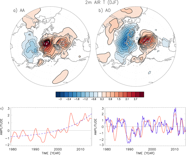
Figure 1. (Upper panels) The DJF patterns of SAT (K) for the first CSEOF mode (a) and the second CSEOF mode (b) in the Northern Hemisphere extratropics poleward of 30° N. (Lower panels) Corresponding amplitude time series with an exponential curve fitted to the first PC time series (blue dashed) and the ±12-month moving averaged AO index time series (blue solid; sign reversed) superposed for the second PC time series (c) and (d).
Download figure:
Standard image High-resolution imageThe second CSEOF mode, explaining ∼8.7% of the total SAT variance, depicts significant warm anomalies over the northern part of North America and North Atlantic and cold anomalies over the northern Eurasia. This SAT pattern is quite similar to that associated with the negative AO (see figure 10 of Thompson and Wallace (2000)). In fact, the corresponding amplitude time series bears a strong resemblance with the ±12-month moving-averaged AO index with a correlation of 0.65 (0.71 with DJF only). Therefore, this mode is called the AO mode in this study (see also figures S2 and S3). The anomalous SAT patterns are most conspicuous in winter (see figure S2). As will be discussed below, the Eurasian SAT patterns associated with these two leading CSEOF modes bear striking resemblance with those of Mori et al (2014).
Physically consistent patterns of sea ice, heat flux, longwave radiation, and 1000 hPa geopotential height/wind for the first and second CSEOF modes are further depicted in figures 2 and 3, respectively. For the AA mode, a significant sea ice loss is seen in the region of anomalously warm SAT (e.g., Barents–Kara Seas). Consistent with this, SST is anomalously warm in the vicinity of sea ice loss, and a significant amount of sensible heat flux and, to a lesser extent, latent heat flux is released from the sea surface exposed to cold air. Previous studies suggest that the increased turbulent heat flux through the exposed sea surface enhances atmospheric warming, which in turn accelerates sea ice melting (Serreze et al 2009, Screen and Simmonds 2010a, 2010b). On the other hand, anomalous turbulent heat flux is negative in the North Atlantic, where SIC anomalies are not significant, probably due to the warming of the atmospheric column in association with AA and the decreased temperature contrast between the sea surface and the overlying air. Further, weak net upward longwave radiation is observed in the reduced SIC region, whereas net downward longwave radiation is significant over the North Atlantic.
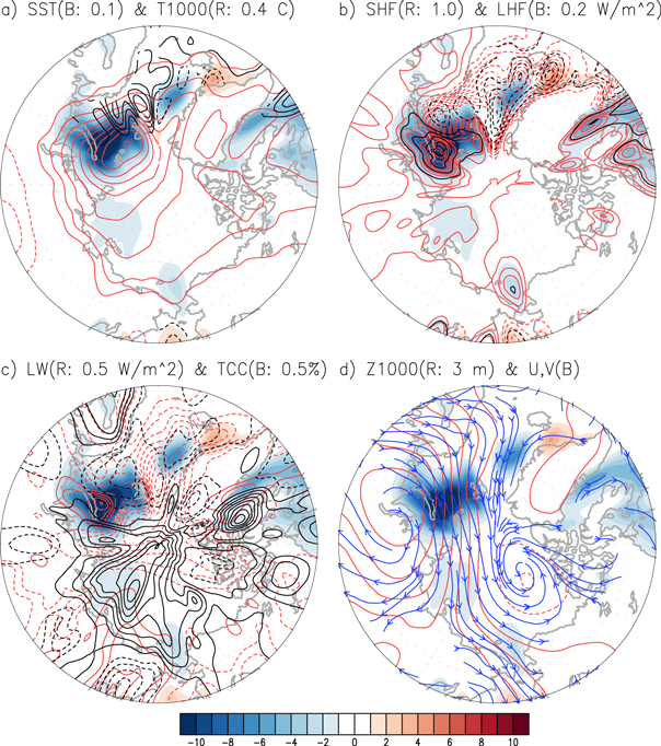
Figure 2. The physical characteristics of the AA mode: wintertime (DJF) anomalous patterns in (60°–90° N) domain of (a) 1000 hPa air temperature (red contours; 0.4 °C), and SST (black contours; 0.1 °C), (b) sensible heat flux (red contour; 1.0 W m−2), and latent heat flux (black contour; 0.2 W m−2), (c) longwave radiation (red contour; 0.5 W m−2) and cloud cover (black contour; 0.5%), and (d) 1000 hPa geopotential height (red contour; 3 m), and streamlines of 1000 hPa wind (blue arrow lines). Positive flux and radiation is upward. In all panels, shading denotes anomalous sea ice concentration (%).
Download figure:
Standard image High-resolution image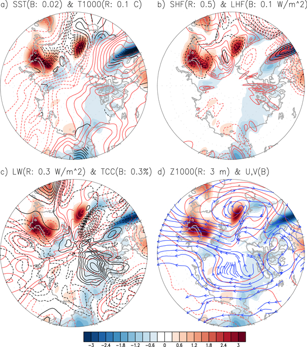
Figure 3. Same as figure 2 but for the negative AO mode. Note that contour and shading intervals, which are indicated in each panel, are different from those in figure 2.
Download figure:
Standard image High-resolution imageThe atmospheric circulation associated with the AA mode is characterized by anticyclonic circulation centered at the southeast of the Barents–Kara Seas (figure 2(d)). This circulation pattern, which causes cold temperature advection across East Asia mid-latitudes (figure 1(a)), is due to the lower tropospheric warm anomalies over the region of the Arctic sea ice loss (Serreze et al 2009, Screen and Simmonds 2010a, 2010b). The anomalous patterns of geopotential height, temperature and wind are physically consistent in the context of the hydrostatic and thermal wind balances (see figure S4).
During the negative phase of the AO mode, lower tropospheric temperature is anomalously cold in the eastern half and is anomalously warm in the western half of the Arctic (figure 3(a); see also Thompson and Wallace (2000)). In consistence with SAT anomalies, SIC anomalies are positive over the Barents–Kara Seas and the Greenland Sea, although their changes are only ∼1%–3% when the AO index is varied by one standard deviation; this contrasts with a maximum decrease of ∼20% when the AA mode is developed (compare figures 2(a) and 3(a)). Sensible and latent heat flux anomalies in the Arctic are also consistent with SIC and SST anomalies particularly on the eastern side of the North Pacific (figure 3(b)). In general, the sign of net upward longwave radiation is opposite to that of lower tropospheric temperature anomaly, suggesting that upward longwave radiation increases due to anomalously cold tropospheric temperature (figure 3(c)). For the atmospheric circulation, anticyclonic circulation over the Atlantic sector is evident (figure 3(d)). This circulation pattern seems consistent with the sea ice anomaly in the Barents–Kara Seas. The resulting northerly and cold temperature advection explains cold SAT anomalies in the northern part of the Eurasian continent (figure 1(b)). It appears that change in total cloud cover is not significantly correlated with the sea ice reduction in the Barents–Kara Seas (figures 2(c) and 3(c)). On the other hand, it should be mentioned that the present generation of numerical models does not simulate cloud cover accurately.
It is worthy to note that the AO-related SIC anomalies over the Barents–Kara Seas (figure 3(a)) are somewhat different from what expected from earlier studies. As introduced previously, the negative AO in winter has often been related with the Arctic sea ice loss in autumn (Overland et al 2011, Cohen et al 2014). Indeed, the AO mode seems to be linked with the sea ice loss in autumn (see figure S6). In winter, however, the negative phase of the AO is related with a slight increase (not decrease) of SIC. It appears that the decreased SAT over the eastern half of the Arctic in winter during the negative phase of the AO increases SIC particularly over the Barents–Kara Seas. This contrasts to the AA mode which is related with the Arctic sea ice loss in all seasons (see figure S5).
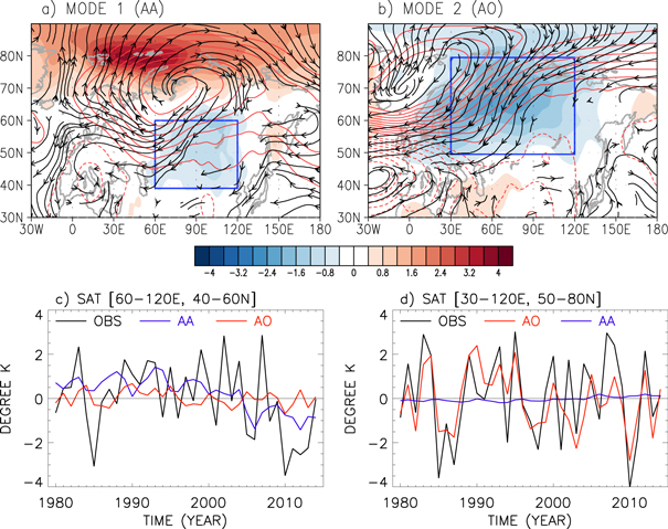
The winter (DJF) patterns of SAT, 1000 hPa geopotential height and stream function anomalies associated with the AA and AO modes are further illustrated in figures 4(a) and (b) for the Eurasian domain. To be consistent with the cold SAT in the mid-latitudes, the negative AO is considered in figure 4(b). The mid-latitude SAT patterns induced by these two modes are again very distinct. One notable difference is the opposite sign of SAT in the Eurasian high-latitudes north of ∼70° N. Another striking difference is the center of the anticyclonic circulation. While the AA mode has a circulation center at around [80° E, 70° N], the AO mode has a center at [0°, 75° N]. Because of the opposite SAT anomalies in the Arctic region, the anomalous SIC in the Barents–Kara and Chukchi Seas as well as the associated lower tropospheric change are also opposite in sign between the AA and the AO modes (see also figures 2 and 3). Further, weak negative SAT anomalies in the AA mode are confined to the region of [60°–120° E × 40°–60° N], whereas those due to the AO mode are widespread in the region of [30°–120° E × 50°–80° N].
Figure 4. (a), (b) Anomalous circulations and temperature patterns associated with the AA mode (a) and negative AO mode (b): temperature (shadings, K), 1000 hPa geopotential (red contours, m2 s−2), and 1000 hPa streamfunction (black arrow lines). (c), (d) Winter (DJF) averaged 2 m air temperature from the raw data (black) and that from the AA mode (red) and the AO mode (blue) over the domain (c) [60°–120° E × 40°–60° N] and (d) [30°–120° E × 50°–80° N]. Year 1979, for example, represents December 1979–Feburay 1980.
Download figure:
Standard image High-resolution image
Figures 4(a) and (b) clearly indicate that the regions affected by the two CSEOF modes differ substantially, and this difference should be taken into account when examining the Eurasian winter SAT anomalies. Figures 4(c) and (d) show the winter SAT anomaly from 1979/1980 to 2013/2014 averaged over the domains [60°–120° E × 40°–60° N] and [30°–120° E × 50°–80° N], respectively. The SAT variation associated with the AA mode is correlated at 0.50 with the raw winter temperature anomaly averaged over the mid-latitude East Asia and explains ∼25% of the total variance. The AO mode plays a minimal role in this region. On the other hand, the AO mode is correlated at 0.69 with the raw winter temperature anomaly averaged over the high-latitude Eurasia and explains ∼53% of the total variance, while the AA mode explains little of the temperature variability in this region. This result suggests that the relative importance of the AA and AO modes on Eurasian SAT anomalies is highly sensitive to the region of interest. For example, 2005/06 cold winter in mid-latitude East Asia [60°–120° E × 40°–60° N] was primarily associated with the AA mode and was not likely linked with the AO mode in any significant manner (figure 4(c)). On the other hand, 2009/10 cold winter over the high-latitude Eurasia [30°–120° E × 50°–80° N] was likely related with the negative AO mode (figure 4(d)). It should be noted that the AA mode in figure 4(c) explains primarily the long-term trend, whereas the AO mode in figure 4(d) explains the seasonal variability. Thus, the AO is a dominant factor for year-to-year variability while the AA explains the general cooling trend over Eurasia in recent years.
4. Discussion
In this study, the two leading modes of winter SAT variability in the Northern Hemispheric extratropics are identified; i.e., AA mode that is associated with the accelerated warming and sea ice melting in the Arctic region, and AO mode that represents SAT variability associated with the intrinsic (natural) variability. These two modes together explain ∼24% of total SAT variability in the Northern Hemisphere north of 20° N. The associated SAT patterns are distinctly different. While the AA mode exhibits a warm Arctic-cold Eurasia pattern, the AO mode shows a widespread monopole pattern with cold Eurasia during its negative phase. Cold Eurasian winters in the recent decades are caused by these two modes, but their relative importance is dependent on the region of interest.
The two leading modes identified in this study are qualitatively similar to those in Mori et al (2014). Mori et al separated the two leading modes by performing EOF analysis. Their first mode represents the AO, while the second mode resembles the AA mode in the present study; the order of the two modes is switched. This difference is likely results from the methodology. While Mori et al used seasonal-mean SAT over the Eurasian domain, monthly-mean SAT anomalies over the whole Northern Hemisphere extratropics, north of 20° N, is considered without seasonal averaging in this study.
More importantly, the present study provides the physical characteristics of the AA and AO modes, which were not explored in Mori et al (2014). The AA mode is associated with the Arctic sea ice loss, centered at the Barents–Kara Seas, and the enhanced turbulent heat flux from the exposed sea surface. In response to anomalously warm lower troposphere, positive geopotential height anomalies develop to the southeast of the Barents–Kara Seas. This anticyclonic circulation advects cold Arctic air into mid-latitude East Asia, resulting in cold winters. The negative AO mode, on the other hand, results in anomalously cold SST in the North Atlantic and enhanced SIC in the Barents and Kara Seas. Further, sea ice anomaly related to the AO mode is about an order of magnitude smaller than that associated with the AA mode. Positive geopotential height anomalies develop in the North Atlantic side of the Arctic, leading to anomalous northerly and cold temperature advection in the mid-to-high latitude central Eurasia.
Acknowledgments
This research was supported by the Korea Meteorological Administration Research and Development Program under Grant KMIPA 2015-2100 and Korea Ministry of Environment as 'Climate Change Correspondence Program'. KYK acknowledges support by SNU-Yonsei Research Cooperation Program through Seoul National University in 2015.