

Abstract
We compare life cycle greenhouse gas (GHG) emissions from several light-duty passenger gasoline and plug-in electric vehicles (PEVs) across US counties by accounting for regional differences due to marginal grid mix, ambient temperature, patterns of vehicle miles traveled (VMT), and driving conditions (city versus highway). We find that PEVs can have larger or smaller carbon footprints than gasoline vehicles, depending on these regional factors and the specific vehicle models being compared. The Nissan Leaf battery electric vehicle has a smaller carbon footprint than the most efficient gasoline vehicle (the Toyota Prius) in the urban counties of California, Texas and Florida, whereas the Prius has a smaller carbon footprint in the Midwest and the South. The Leaf is lower emitting than the Mazda 3 conventional gasoline vehicle in most urban counties, but the Mazda 3 is lower emitting in rural Midwest counties. The Chevrolet Volt plug-in hybrid electric vehicle has a larger carbon footprint than the Prius throughout the continental US, though the Volt has a smaller carbon footprint than the Mazda 3 in many urban counties. Regional grid mix, temperature, driving conditions, and vehicle model all have substantial implications for identifying which technology has the lowest carbon footprint, whereas regional patterns of VMT have a much smaller effect. Given the variation in relative GHG implications, it is unlikely that blunt policy instruments that favor specific technology categories can ensure emission reductions universally.
Export citation and abstract BibTeX RIS
1. Introduction
Past studies have shown that life cycle plug-in electric vehicle (PEV) emissions depend heavily on the assumed electricity grid mix [1–7], driving patterns (including drive cycle and distance) [8–10] and climate (including ambient temperature) [7, 11]. These factors vary regionally, so PEV emissions implications also vary regionally. Several studies have assessed regional differences in PEV emissions incorporating subsets of these factors [2, 4–7, 11–15]—with most focused on regional grid mix, but no study has accounted for the combined influence of consequential grid emissions, driving patterns, and temperature heterogeneity in assessing regionally-specific life cycle implications of PEVs in the US. In table 1 we summarize studies that make regional comparisons of PEV emissions in the United States. Key factors that differentiate these studies include:
Table 1. Summary of published studies assessing the regional variation in electrified vehicle GHG emissions in the United States.
| Study | Vehicle types | Regional resolution | Life cycle scope | Electricity source and emissions | Utility factor or VMT pattern | Driving conditions | Temperature |
|---|---|---|---|---|---|---|---|
| EPRI-NRDC (2007) [14] | PHEV | NERC regions | Use Phase | Consequential | Homogeneous | Homogeneous | Ignored |
| Electricity upstream and generation; gasoline upstream and combustion | Bottom-up modeled emissions (573 g CO2e kWh−1 in 2010; 97–412 g CO2e kWh−1 in 2050) | (PHEV10: 0.12 PHEV20: 0.49 PHEV40: 0.66) | Federal Urban Driving Schedule (FUDS) | ||||
| Hadley and Tsvetkova (2009) [15] | PHEV | 13 NERC subregions | Partial Use Phase | Consequential | Homogeneous | Homogeneous | Ignored |
| Electricity generation; gasoline combustion | Bottom-up approach using ORCED model assuming 25% PHEV market penetration by 2020 | Not clear | Three load levels assumed per vehicle—1.5 kW, 2 kW, and 6 kW | ||||
| Anair and Mahmassani (2012) [4] | ICV, HEV, PHEV, BEV | eGRID subregion | Use Phase | Attributional | Homogeneous | Homogeneous | Ignored |
| Electricity upstream and generation; gasoline upstream and combustion | Average regional generation covering transmission and upstream loss (286–983 gCO2e kWh−1) | (Chevrolet Volt: 0.64) | EPA combined driving cyclea | ||||
| MacPherson et al (2012) [17] | PHEV | NERC regions, NERC | Life Cycle | Attributional | Homogenous: | Homogenous | Ignored |
| subregions and states | Average regional and state based emissions from EPA eGRID2010 database | PHEV35: 0.635, andRegional: NERC region based utility factors estimated based on NHTS. | EPA combined driving cycle | ||||
| Thomas (2012) [19] | HEV, PHEV, BEV | 13 NERC subregions | Use Phase | Consequential | Not clear | Not clear | Ignored |
| Electricity upstream and generation from GREET; gasoline well-to-wheel using GREET (2001) | Average marginal emissions from Hadley and Tsvetkova (2009) | ||||||
| Yawitz et al (2013) [13] | HEV, PHEV, BEV | State | Life Cycle | Attributional | Homogeneous | Homogeneous | Ignored |
| Average state generation | PHEV: 0.5 | EPA 2013 | |||||
| Graff Zivin et al (2014) [5] | ICV, HEV, PHEV, BEV | eGRID subregion | Partial Use Phase | Consequential | Homogeneous | Homogeneous | Ignored |
| Electricity generation; gasoline combustion | Marginal NERC emissions considering interregional trading | 35 mi day−1 | EPA combined city/highway | ||||
| Onat et al (2015) [6] | ICV, HEV, PHEV, BEV | 13 NERC subregions | Life Cycle | Consequential | Regional | Homogeneous | Ignored |
| Marginal emissions from Thomas (2012) [19] which is based on ORCED model | State based utility factors | EPA combined | |||||
| Tamayao et al (2015) [2] | ICV, HEV, PHEV, BEV | NERC region | Life Cycle | Consequential | Homogeneous | Homogeneous | Ignored |
| Compares Graff Zivin et al (2014) and Siler-Evans et al (2012) marginal emission factors by NERC region and average state, eGRID subregion, and NERC emission factors | US NHTS (2009) national distribution | EPA combined | |||||
| Yuksel and Michalek (2015) [11] | BEV | NERC region | Partial Use Phase | Consequential | Homogeneous | Homogeneous | Regional |
| Electricity generation; gasoline combustion | Compares Graff Zivin et al (2014) and Siler-Evans et al (2012) marginal emission factors by NERC region. | US NHTS (2009) national distribution | Efficiency based on FleetCarma on-road data [28] | Based on FleetCarma data for Nissan Leaf and regional temperature data | |||
| Nealer et al (2015) [18] | BEV | eGRID subregions | Life Cycle | Attributional | Homogeneous | Homogeneous | Ignored |
| Average emission rate for generators located in each subregion. | EPA combined city/highway | ||||||
| Archsmith et al (2015) [20] | ICV, BEV | NERC regions | Life Cycle | Consequential | Regional | Homogeneous | Regional |
| Regression-based marginal emission estimates for current, average emission rates for future | Based on regional NHTS data | Based on GREET | Based on data from [26–27] | ||||
| This study | ICV, HEV, PHEV, BEV | County-level estimates | Life Cycle | Consequential | Regional | Regional | Regional |
| based on highest-resolution data available for each factor | Compares Graff Zivin et al (2014) and Siler-Evans et al (2012) marginal emission factors by NERC region. | NHTS (2009) state distribution | EPA city, highway or combined based on county urbanization level | Based on ANL temperature-controlled laboratory test data and regional temperature data. |
aThe US Department of Energy define three driving conditions: city—'urban driving, in which a vehicle is started in the morning (after being parked all night) and driven in stop-and-go traffic'; highway—'a mixture of rural and interstate highway driving in a warmed-up vehicle, typical of longer trips in free-flowing traffic'; (3) combined—'combination of city driving (55%) and highway driving (45%)' [48].
1.1. Life cycle scope
Existing studies assessing PEV emissions have different life cycle scopes, which may include or exclude each of the following: vehicle and battery manufacturing emissions; gasoline extraction, processing, transportation, and fuel combustion emissions; power plant emissions from electricity generation for vehicle charging; power plant fuel feedstock extraction, production and transportation emissions; and end of life emissions. Several of the studies shown in table 1 only include emissions related to vehicle use or a subset of the emissions related to vehicle use (e.g., vehicle tailpipe emissions and power plant smokestack emissions), leading to incomplete assessments. Life cycle studies suggest that emissions implications from sources other than tailpipe and power plant emissions can comprise one fifth to one third of vehicle life cycle greenhouse gas (GHG) emissions [2, 6, 16, 17], so addressing the full life cycle can be important for comprehensive comparisons.
1.2. Electricity sources and emissions
Critical to assessing life cycle emissions of PEVs are the sources of energy used to generate electricity and their efficiencies [1, 2, 4, 5, 7, 12, 13]. While some studies use an attributional life cycle approach in which they assign to the PEV the average emission rates for power plants in the same state or power grid region where it is charged [4, 13, 17, 18], other studies take a consequential life cycle approach, estimating the change in grid emissions resulting from new PEV charging in a region [5, 7, 14, 15, 19]. The latter is appropriate for assessing the emissions implications of a policy intervention. One empirical approach to estimating consequential emissions of PEV charging is to estimate marginal emission factors using historical data. Several studies have conducted regressions on past data to estimate marginal emission rates for US grid regions [5, 20, 7], though Alexander et al (2015) warn that regional marginal emissions can be difficult to identify because of interregional trade [21]. Tamayao et al (2015) [2] show that differences between average and marginal emission factors can affect whether PEVs are estimated to be higher or lower emitting than efficient gasoline vehicle models. In some cases, the uncertainty is such that one is not able to conclude whether the emissions from PEVs are larger or smaller than efficient gasoline vehicle models.
1.3. Driving patterns
Driving conditions (specifically, driving cycle—the trajectory of vehicle velocity over time) can affect the relative vehicle efficiency of PEVs and conventional gasoline vehicles differently and thus substantially affect the relative economic and environmental benefits of electrified vehicles. For instance, PEVs can offer substantial economic and GHG benefits over conventional vehicles (CVs) for stop-and-go city driving while offering fewer environmental benefits at a higher cost premium for highway cruising [8]. Patterns of driving distance also matter, particularly for PHEVs, which use a mix of gasoline and electricity for propulsion. For example, longer driving distances lead to higher petroleum and total energy use [9, 10], and the shorter distances traveled by urban drivers result in higher PHEV utility factors [22]. As shown in table 1, most existing studies have modeled regional heterogeneity of electricity source but ignore regional differences in driving distance distributions and driving conditions that affect vehicle efficiency.
1.4. Temperature
Most studies ignore the regional effect of ambient temperature. However, temperature has an important effect on vehicle efficiency due to heating, ventilation, and air conditioning (HVAC) use and temperature-related battery efficiency effects. Indeed, compared to mild regions, Yuksel and Michalek (2015) [11] estimate that battery electric vehicles (BEVs) can consume an average of 15% more energy in hot and cold regions of the US. Similarly, Neubauer and Wood (2014) [23] estimate that HVAC use can increase energy consumption by 24% in cold climates, and Kambly and Bradley (2014) [24, 25] note that HVAC use can decrease BEV range depending on the region and time of day; and Meyer et al (2012) [26] observe a 60% drop in range in −20 °C lab tests with maximum climate control use. Archsmith et al (2015) [7] use vehicle test data from Meyer et al (2012) [26] and Lohse-Busch et al (2013) [27] to argue that temperature can have as large an effect on electric vehicle charging emissions as regional grid mix, and in a working paper Holland et al (2015) [12] adjust vehicle efficiency regionally to account for temperature effects in estimating air pollution damages.
To assess the combined effect of these regional factors, we develop and apply a model that integrates the effects of electricity source, driving patterns, and temperature with a comprehensive life cycle scope to characterize regional GHG emissions from electricity and gasoline light-duty vehicles.
2. Data and methods
We perform a comparative life cycle assessment of the CO2 emissions across five existing vehicle models summarized in table 2. These vehicle models represent CVs, hybrid electric vehicles (HEVs), plug-in electric vehicle (PHEVs), and BEVs, and they were selected based on availability of Argonne National Laboratory vehicle test efficiency data at high, low, and moderate test chamber temperatures [29].
Table 2. Vehicle models considered.
| Vehicle model | Type | Model year | Battery energy capacity | |
|---|---|---|---|---|
| Nominal (kWh) | Usable (kWh) | |||
| Nissan Leaf | BEV | 2013 | 24 | 21 |
| Chevy Volt | PHEV (EREV) | 2013 | 16.5 | 10.8 |
| Toyota Prius PHEV | PHEV (blended) | 2013 | 4.4 | 2.7 |
| Toyota Prius | HEV | 2010 | — | — |
| Mazda 3 (with i-ELOOP) | CV | 2014 | — | — |
Figure 1 summarizes the framework used in this work. We start by assigning driving conditions to each county based on urbanization level; we assign vehicle miles traveled (VMT) patterns to counties based on data from the National Household Travel Survey (NHTS) for the corresponding state; and we assign marginal grid emission factors for each North American Electric Reliability Corporation (NERC) region to the counties that lie in that region. We then estimate the energy consumption rate for each vehicle based on Argonne National Laboratory's Downloadable Dynamometer Database (D3) temperature-controlled chamber vehicle test data together with information on temperature, drive cycle, and VMT patterns for each county. We use energy consumption and VMT patterns to compute timing and duration of vehicle charging. Finally, we estimate life cycle CO2 emissions for each vehicle type and location by adding vehicle and battery manufacturing emissions, gasoline combustion and upstream emissions (based on computed gasoline consumption), and electricity production and upstream emissions (based on computed electricity consumption, timing, and location).
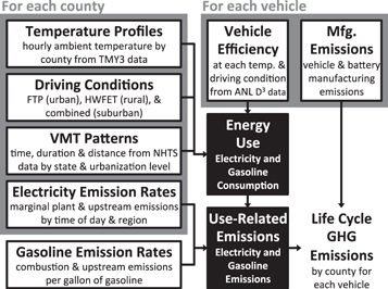
Figure 1. Framework for the analysis.
Download figure:
Standard image High-resolution imageWe use county-level data when such resolution exists, and we use regional data where we lack county-level resolution. We perform sensitivity analysis to test implications of several factors and assumptions and to test robustness of our results. We explain each of these modules in the following sections with additional detail provided in the SI.
2.1. Vehicle energy efficiency
For each vehicle model in table 2 we estimate how vehicle energy efficiency changes with driving cycle and temperature. We use the D3 database from Argonne National Laboratory's Advanced Powertrain Research Facility [29], which provides dynamometer test data for several vehicle models. D3 provides energy efficiency estimates at three different temperatures (20° F, 72° F and 95° F) and for three different standard test driving cycles (the urban dynamometer driving schedule (UDDS) cycle, the US06 cycle, and the highway fuel economy test (HWFET) cycle) [30]. During the tests at 20° F and 95° F, the climate control is set to keep the cabin temperature at 72° F. These '2-cycle' tests, used in federal regulatory compliance calculations, are known to produce optimistic fuel consumption results relative to on-road driving, resulting in lower than actual emission estimates [31]. We use linear interpolation between each measured point, and we avoid extrapolation below 20° F and above 95° F (instead holding the efficiency estimate fixed at the corresponding extremum for temperatures outside the measured ranges). The measured efficiency estimates account for charging losses.
2.2. VMT patterns
Daily trip length and timing for light-duty vehicles in each county is drawn from the distribution of trips in the NHTS [32] from all counties from the same state from a set of 76 149 total vehicles (we filter the dataset to private light-duty vehicles only and exclude the data points that are reported by members of the household other than the driver). Trip details are used to account for the ambient temperature effect (as temperature varies through the day) and to assess when the vehicle is available for charging. We test alternative assumptions in the sensitivity analysis.
2.3. Driving conditions
For urban counties we use the UDDS test results; for rural counties we use the HWFET cycle results; and for outlying (suburban) counties we use the combined results to represent the dominant driving conditions in each case. We test alternative assumptions in the sensitivity analysis.
2.4. Charging profile
We assume convenience charging, i.e., charging starts as the last trip of the day ends. We estimate the charging duration based on the daily energy consumption of each vehicle. We test alternative assumptions in the sensitivity analysis.
2.5. Temperature
We use the Typical Meteorological Year (TMY3) Database from the National Renewable Energy Laboratory [33] which provides hourly ambient temperature data for a typical meteorological year for 1011 locations in the continental United States. We use a triangulation-based linear spatial interpolation method [34] to estimate temperature profiles at the center of each county. In the sensitivity analysis, we assess the effect of ignoring temperature on our results.
2.6. Emission factors
For electricity emissions associated with PEV charging, we use the 2011 marginal emission factors from Siler-Evans et al [20], which are based on regressions of empirical, historical changes in power plant emissions with respect to changes in generation within each NERC region. We examine this choice in more detail in the discussion section and test alternative assumptions in the sensitivity analysis.
Table 3 summarizes emissions estimates associated with manufacturing and assembly of vehicles and lithium-ion battery packs; gasoline production, transport and combustion; and electricity upstream, production, transmission, and distribution.
Table 3. Assumptions and data sources used for each life cycle stage.
| Emissions source | Estimate(s) used | Data source |
|---|---|---|
| Vehicle manufacturing (including battery) | 18 g mi−1 CV | GREET (2013) [35] and Tamayao et al (2015) [2] |
| 16 g mi−1 HEV | ||
| 41 g mi−1 PHEV-EREV | ||
| 22 g mi−1 PHEV-blended | ||
| 51 g mi−1 BEV | ||
| Gasoline combustion | 8655 gCO2 gal−1 gasoline | Average of values from EPA (2014) [36] and Venkatesh et al (2011) [37] |
| Gasoline production and transportation | 2400 gCO2 gal−1 gasoline | Average of values from Venkatesh et al (2011) [37] and GREET (2013) [35] |
| Electricity generation | 430–932 kgCO2eq MWh−1 | Siler-Evans et al (2012) [20] |
| Electricity upstream | 38–107 kg CO2 MWh−1 | Tamayao et al (2015) [2] (estimated based on Siler-Evans et al (2012) [25] Graff Zivin et al (2014) [5], Venkatesh et al (2011) [37], Venkatesh et al (2011) [38], and US EPA (2009) [39]) |
3. Results and discussion
Figure 2 summarizes the increase or decrease in life cycle GHG emissions from driving a 2013 Nissan Leaf BEV, a 2013 Chevrolet Volt PHEV, or a 2013 Toyota Prius PHEV relative to the most efficient gasoline vehicle in the market—the Toyota Prius HEV (modeled here using data from a 2010 HEV Prius)—and relative to a CV of comparable size—the Mazda 3. A map of county urbanization level is provided in the SI, since urbanization level determines drive cycle.
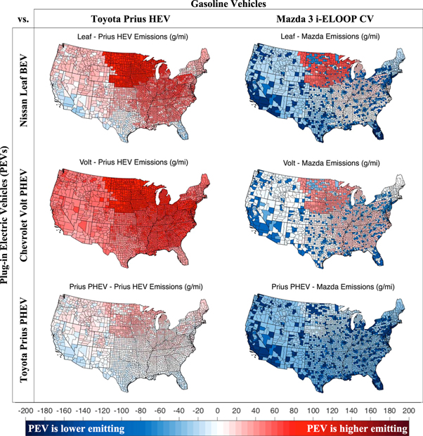
Figure 2. Estimated difference in life cycle GHG emissions (gCO2eq mi−1) of selected plug-in electric vehicles (2013 Nissan Leaf BEV, 2013 Chevrolet Volt PHEV, and 2013 Prius PHEV) relative to selected gasoline vehicles (2010 Prius HEV and 2014 Mazda 3). In each case blue indicates that the PEV has lower GHG emissions than the gasoline vehicle and red indicates that the PEV has higher GHG emissions than the gasoline vehicle.
Download figure:
Standard image High-resolution imageThe Nissan Leaf BEV produces lower life cycle GHG emissions than the Prius HEV in urban counties of Texas, Florida, and much of the southwestern US. In most of the rest of the country the Leaf increases GHG emissions relative to the Prius HEV, with those increases being most notable in the Midwest and in the South. This is due to the combined effect of grid carbon intensity, highway driving, and regional temperature. In particular, the Northern Midwest has a combination of a coal-heavy electricity grid, rural counties (with an assumed highway driving cycle), and cold weather that all contribute to higher relative emissions for the BEV.
The Chevrolet Volt PHEV has higher life cycle emissions than the Prius HEV in all counties. This is because the Volt consumes more gasoline per mile in charge-sustaining mode (after the battery is depleted) than the Prius HEV, and it consumes more electricity per mile than the Leaf in charge-depleting (CD) mode (when the battery is charged) at high temperatures. Further, in cold weather the Volt consumes both gasoline and electricity in CD mode. Comparison of electricity and gasoline consumption for different vehicles is provided in the SI (section 4).
The PHEV Prius produces lower life cycle GHG emissions than the HEV Prius in Texas, Florida, and the southwestern US as well as in most urban areas, but it produces higher emissions in many rural areas across the country—especially in the Northern Midwest. This is because the PHEV Prius consumes less gasoline than the HEV Prius in city driving conditions and more gasoline than the HEV Prius in highway driving conditions. Differences between the HEV Prius and the PHEV Prius are generally less pronounced than those comparing the HEV Prius to the Volt or the Leaf.
In the right-hand column in figure 2 we provide a similar analysis using a conventional gasoline vehicle, the 2014 Mazda 3 (with i-ELOOP), with EPA-rated combined (5-cycle) fuel efficiency of 32 mpg as the reference vehicle in place of the HEV Prius. The i-ELOOP is an energy recovery braking system intended to capture a portion of the benefits that HEVs and PEVs capture in regenerative braking to displace accessory load without a full hybrid system. Relative to the Mazda 3, we find that (1) the Leaf reduces GHG emissions in urban counties across the US as well as suburban and rural counties in Texas, Florida, the Western US, and New England while increasing GHG emissions in the rural Midwest; (2) the Volt reduces GHG emissions in urban counties across the US while increasing GHG emissions in rural counties of the Midwest and the South; and (3) the Prius PHEV reduces emissions in all counties. In all three cases the GHG emission reductions in urban counties can be substantial.
Figure 3 shows the breakdown of life cycle CO2 emissions for each vehicle in various selected counties from two NERC regions: the Western Electricity Coordinating Council (WECC) and the Midwest Reliability Organization (MRO), which have, respectively, the lowest and highest electricity generation CO2 emissions factors in the continental US. The counties selected within those regions also have diverse climate and urbanization levels. Tailpipe and power plant emissions make up 64%–80% of life cycle GHG emissions in these examples. Batteries are less efficient when cold, and so are engines, but gasoline vehicles are able to use waste heat from the engine to heat the cabin, while BEVs and EREV PHEVs need to draw energy from the battery to heat the cabin, so PEVs tend to have larger energy penalties in cold weather regions than conventional gasoline vehicles.
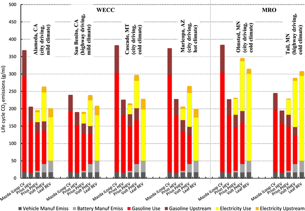
Figure 3. Life cycle CO2 emissions in gCO2eq mi−1 in selected counties. Vehicles are ordered from lowest to highest degree of electrification.
Download figure:
Standard image High-resolution imageThe following conclusions can be made from figure 3:
- The effects of regional climate and grid mix on emissions become more important for vehicles with higher degrees of electrification. We find all vehicles have higher emissions in Minnesota, a colder state, compared to California. However, the increase in emissions is largest for the Leaf BEV, whereas only a slight increase is observed with Mazda 3 CV.
- In contrast, the effect of driving cycle on emissions becomes more prominent for vehicles with lower degrees of electrification. In counties with similar climate conditions and grid mix, we observe that the biggest change in emissions with highway driving compared to city driving occurs with Mazda 3.
- Hot temperatures in Arizona do not increase the emissions from the Leaf significantly relative to mild climate counties in California—an apparent contradiction to Yuksel and Michalek [11], who show a 22% increase in Leaf emissions in hot regions of Arizona compared to coastal California. The primary reason is that the laboratory data used in this study suggest lower energy consumption at high temperatures compared to real world data used in Yuksel and Michalek [11]. Further discussion of this issue is provided in the SI, section 4.
4. Sensitivity analysis
Details regarding the sensitivity analysis can be found in the SI, and table 4 summarizes key findings. Overall, we find that ignoring regional heterogeneity of temperature or driving conditions (city/highway) affects carbon footprint technology comparisons substantially in some regions, whereas urban/rural heterogeneity of VMT patterns has a negligible effect. We also find, consistent with prior work [2], that delayed charging increases the GHG emissions associated with PEVs in most regions and reduces the potential for emissions savings when compared to gasoline vehicles.
Table 4. Summary of findings from the sensitivity analysis.
| Sensitivity case | Change from base case | Purpose | Finding |
|---|---|---|---|
| Homogeneous temperature | Vehicle efficiency at 72° F used for all counties all year | Test importance of temperature effect | Temperature effect substantially changes comparison results for northern states |
| Homogeneous driving conditions | Vehicle efficiency on combined UDDS/HWFET used for all counties | Test importance of drive cycle | Drive cycle affects the relative benefits of PEVs versus HEVs (and especially versus CVs). Without differentiated drive cycles, urban counties are not distinct from nearby rural counties. |
| VMT clustered by state and urbanization level | Each county's VMT distribution is drawn from all NHTS data from the same state and urbanization level | Test importance of differences in urban/rural driving distance | Using MSA level VMT does not change the results significantly. The maximum change is around 2 g mi−1. |
| Delayed charging | Each PEV's charging schedule begins at midnight, rather than upon arrival at home | Test importance of charge timing | Delayed charging increases GHG emissions of PEVs in most of the country and reduces competitiveness with the HEV. |
Figure 4 summarizes life cycle GHG emission results for the Nissan Leaf in six counties. The Minnesota counties, which have both cold weather and the most carbon-intensive electricity grid region, have notably higher life cycle emissions than other counties, and the sensitivity case ignoring temperature has the largest effect on results.
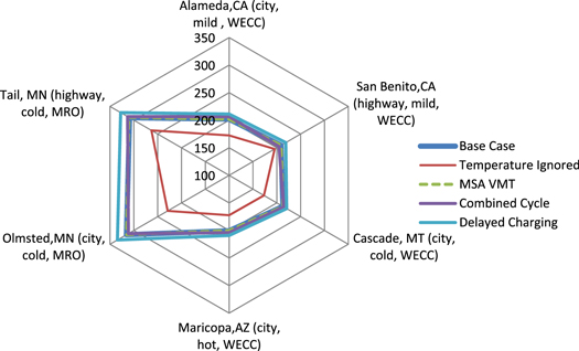
Figure 4. Radar chart showing Nissan Leaf life cycle emissions in gCO2eq mi−1 from different cases in selected counties.
Download figure:
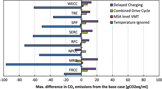
Standard image High-resolution imageFigure 5 summarizes the maximum change in GHG emissions per mile for a Nissan Leaf across all counties for each NERC region between the base case scenario and each sensitivity scenario. Ignoring temperature has the largest effect, reducing emissions estimates by up to 97 gCO2eq mi−1, while ignoring differences in drive cycle can increase emissions in some counties by up to 8 gCO2eq mi−1 (drive cycle affects CV efficiency more than PEV efficiency). Delayed charging can increase Leaf emissions by up to 21 gCO2eq mi−1, while use of MSA-level VMT patterns changes results less than 3 gCO2eq mi−1.
Figure 5. Maximum change in emissions for a Nissan Leaf relative to the base case. The maximum difference is observed in a different county for each case.
Download figure:
Standard image High-resolution image
5. Limitations
Where possible, our analysis uses the most recent data available at the highest resolution available to account consistently for regional effects of grid emissions, driving patterns, and temperature on life cycle GHG emissions of PEVs and gasoline vehicles. However, there are several limitations regarding the data that should be understood when interpreting our results:
5.1. Regional grid emissions
The marginal emissions estimates used in this analysis are based on regressions for year 2011 and may not capture changes that may occur in the grid due to changes in policies, fuel prices, economic conditions or other factors. It is generally expected that GHG grid emission rates will decline over time, during the period that PEVs are being adopted and used. However, consequential (marginal) emissions from new load do not decrease linearly with average grid emission rates. Because marginal emissions come primarily from fossil fuel plants, the mix of natural gas versus coal on the margin primarily determines the consequential emissions of new PEV charging. If the regions that are currently relying on coal at the margin start switching to natural gas generation used at the margin, then the amount of carbon dioxide savings from vehicle electrification will increase, and we may expect the more emissions-intensive areas of the country to look more like the less emissions-intensive areas in the future. Also, while we discuss county-level differences, we implicitly assume that within each NERC region all counties have identical marginal emission factors. Since the electric grid is heavily interconnected, it is difficult to attribute emissions to load changes at county-level resolution. In practice, it may be the case that adding PEV load in some areas of a NERC region could have different emission implications than adding the same load in a different area of the same NERC region.
5.2. Driving patterns
Our summary maps assign the UDDS test results to urban counties and the HWFET test results to rural counties, but in practice driving conditions are heterogeneous in all counties. Also, importantly, on-road driving conditions differ substantively from these two laboratory tests, which are known to produce optimistic fuel efficiency estimates due to their relatively mild drive cycle demands. Driving distances also may vary for different counties in a state, but we lump counties together when estimating driving distance distributions because we lack data resolution to identify driving distance distributions for individual counties. The NHTS data set provides information on the trips taken by each surveyed US vehicle on a single survey day and does not include day-to-day variability for each vehicle. In this study, we average over the vehicle profiles to assess implications for average driving distances and we assume these daily profiles are identical over the year. In practice the driving profiles of PEV adopters may differ from the general population.
5.3. Temperature
We treat temperature as the only factor affecting vehicle efficiency on a particular drive cycle, but in practice other regional factors could affect the results. For example, the level of humidity will affect HVAC use, and the road conditions (such as terrain, precipitation, and wind) can also affect the efficiency of the vehicle. Our efficiency estimates are based on linear interpolation using test results at three temperatures for each drive cycle. Comparisons with in Yuksel and Michalek [11] suggest that this captures the general shape of the trend reasonably well but coarsely. We also avoid extrapolation beyond the range of temperatures tested and therefore likely make optimistic estimates of vehicle efficiency loss in extreme weather regions.
5.4. Vehicles
We examine only five specific vehicle models for which we have access to laboratory test data at multiple chamber temperatures and multiple drive cycles. Other vehicle models, including more recent model years of the vehicles examined, could have different performance characteristics, temperature sensitivity, etc
5.5. Other externalities
We focus on GHG emissions, but other externalities, including criteria air pollutant emissions and their effect on health, dependence on foreign oil and its relation to energy security and independence, water resource use for energy production, and battery hazardous waste disposal play important roles in guiding policy decisions. In particular, electric vehicle externalities from air pollution may be larger then those for global warming [12, 16, 40].
6. Policy implications
Our results suggest that the GHG-reduction benefits of PEVs have significant regional variability due to grid mix, temperature, and driving conditions as well as differences among vehicle alternatives within each technology class. This suggests that a regionally-targeted vehicle-specific strategy to encourage adoption primarily in areas where specific PEVs provide the largest benefits could increase the GHG reductions achievable under a given budget.
While current federal policy for PEVs is fairly uniform across the US, individual states have adopted differentiated policies including zero-emission vehicle mandates, state tax breaks for PEV purchases, and a range of other incentives, such as subsidized charging infrastructure or access to high-occupancy vehicle lanes for PEV owners. For instance, California, Oregon, New York, New Jersey, Maryland, Connecticut, Rhode Island, Massachusetts, Vermont, and Maine all have policies that mandate sales of vehicles with zero tailpipe emissions (called 'zero emission vehicles' or ZEVs) based on California's policy authorized under section 177 of the Clean Air Act [41]. In urban counties (city driving) of these ZEV states the PEVs we model are lower emitting than the Mazda 3 CV, but they are not all lower emitting in rural counties (highway driving), and some PEVs (e.g.: the Volt) are higher-emitting than the gasoline-powered Prius HEV in all counties of these states.
Further, state subsidies for PEV purchases vary, with the largest subsidies offered in Colorado and, until recently, in West Virginia and Georgia [42], and there is evidence that subsidies increase adoption [43]. West Virginia and Georgia in particular are locations where the GHG case for PEVs in our analysis is less strong, since the gasoline-powered Prius HEV has lower life cycle GHG emissions there than either the Leaf BEV or the Volt PHEV.
Our results suggest that the GHG case for PEVs is generally strongest in urban counties of Texas, Florida, and the Southwestern US followed by New England, and it is generally weakest in the Midwest and the South. However, it is important to note that these estimates are uncertain and dynamic, since (1) the power grid is highly interconnected and changes over the life of the vehicle as the power plant fleet and feedstock prices fluctuate, (2) on-road weather effects on vehicle efficiency may differ from controlled laboratory tests at fixed ambient temperature settings, (3) driving conditions in practice are heterogeneous within each county and are far more diverse than the standard city/highway laboratory tests can capture, and (4) PEV benefits relative to gasoline vehicles vary across different PEV models and depend on which gasoline vehicle the PEV buyer would have purchased if the PEV were not available. The complexity of these uncertain and dynamic regional and vehicle differences makes it difficult to forecast regional GHG benefits of PEVs with certainty, and such challenges pose difficulties for regulators worldwide.
Broadly, regional policies that are more aligned with the GHG benefits we estimate could be more efficient at achieving GHG reductions, though other factors such as regional consumer preferences, political climate, and other externalities also affect regional policy choices. In general, policies that target GHG reductions directly, such as carbon tax or cap-and-trade policies, rather than favoring specific technologies, are likely to be more efficient at achieving GHG reductions, though support for the development and deployment of new technologies can also have dynamic benefits and potentially lead to large long-term benefits if they enable a fleet transition that would not have happened otherwise [44, 45]
Regional differences in GHG emissions from PEVs also have implications for vehicle labeling and regulation. GHG emission estimates used for vehicle fuel economy and environment labels (window stickers) currently report only tailpipe emissions. But upstream GHG emissions from PEV charging can be larger than tailpipe emissions, and they vary regionally. Ideally, future labels will include life cycle emissions estimates that include power plant emissions—but this goal is challenging to achieve with precision given the regional variability and the challenges described previously. Secondly, the US EPA regulates GHG emissions from motor vehicle fleets and currently treats PEVs as though they are zero-emission vehicles when operating on electricity [43]. If future regulations are updated to incorporate upstream PEV emissions from vehicle charging, as they are expected to, regional differences and regional patterns of vehicle adoption will be important to achieving meaningful estimates of GHG emissions from PEVs.
Finally, larger factors can influence policy strategies. For example, when deciding where to allocate scarce public resources, benefits of light-duty transportation electrification must be weighed against benefits that could be achieved in other sectors [46]. Further, our analysis focuses on life cycle emissions directly associated with the vehicles we assess and ignores consequential fleet-wide GHG emission effects of PEV adoption due to alternative fuel vehicle incentives in federal corporate average fuel economy policy and GHG emissions standards. These incentives allow automakers that sell PEVs to meet less-stringent fleet GHG emission standards, at least through 2025, result in net GHG increases when PEVs are sold [47]. This policy effect can be large enough to wipe out any net GHG savings offered by PEV adoption in the near term, although PEV adoption could also have dynamic effects on technology trajectories in the light-duty vehicle fleet that help encourage a long term transition.
Acknowledgments
The authors would like to thank Kevin Stutenberg, Eric Rask, and Forrest Jehlik from Argonne National Laboratory for their help with the dynamometer test data. Funding for this work came from a grant from the Engineering Research and Development for Technology Scholarship Program at the University of the Philippines, a gift from Toyota Motor Corporation, and the Center for Climate and Energy Decision-Making (CEDM), through a cooperative agreement between the National Science Foundation and Carnegie Mellon University (SES-0949710 and SES-1463492). The findings and views expressed are those of the authors and not necessarily those of the sponsors.