Transatlantic flight times and climate change

It has long been recognised that aviation affects the climate, through the radiative forcing associated with greenhouse-gas emissions and contrails (Stuber et al 2006, Lee et al 2009). However, it is becoming increasingly clear that the interaction is two-way and that climate change has important consequences for aviation. For example, stronger mid-latitude wind shears in the upper troposphere and lower stratosphere appear to be destabilising the atmosphere and causing clear-air turbulence to intensify (Williams and Joshi 2013). At ground level, warmer air reduces the lift force on the wings of departing aircraft and appears to be increasing the likelihood of take-off weight restrictions (Coffel and Horton 2015). Here we investigate the influence of climate change on flight routes and journey times. This subject has received relatively little attention, but is potentially important because of the acute sensitivity of the commercial aviation sector to fuel costs (Karnauskas et al 2015).

The route between two airports that minimises the distance travelled is the great circle, which is the spherical equivalent of a straight line. However, it is more economical to minimise the journey time than the distance travelled. For this reason, aircraft routinely deviate from the great circle route in a carefully optimised manner, to benefit from tailwinds or avoid headwinds (Lunnon and Marklow 1992). The day-to-day variability of flight routes and journey times is therefore dictated by the horizontal wind field in the atmosphere (Palopo et al 2010). The inter-annual variability of flight routes and journey times between Hawaii and the continental USA has been found to be caused predominantly by anomalous wind patterns associated with the El Niño Southern Oscillation and Arctic Oscillation (Karnauskas et al 2015). Although the North Atlantic flight corridor between Europe and North America is one of the world's busiest, with approximately 600 crossings each day (Irvine et al 2013), little is known about the long-term response of transatlantic flight routes and journey times to the wind changes associated with global warming.

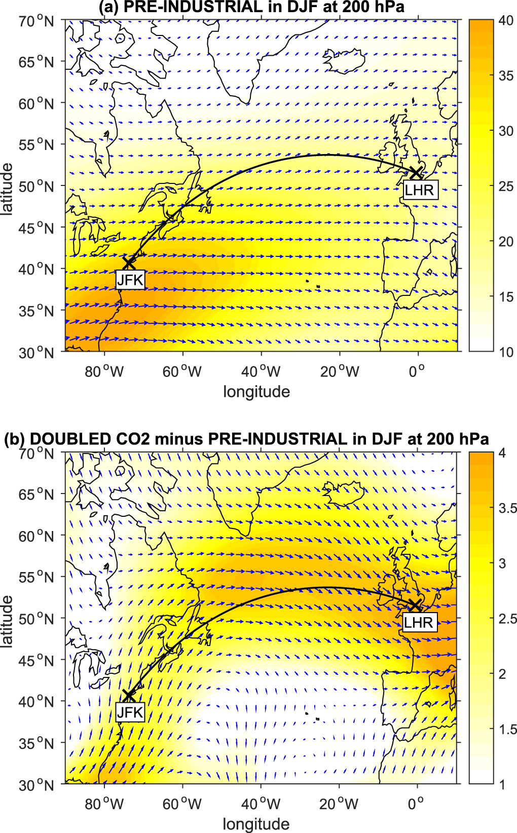
The average wintertime jet-stream winds in the upper troposphere and lower stratosphere of the north Atlantic sector are generally projected to become stronger in response to greenhouse-gas forcing, as shown in figure 1. This strengthening is consistent across the current generation of climate models, although the magnitudes and structures of the strengthening vary in detail from one model to another (Woollings and Blackburn 2012, Haarsma et al 2013). The strengthening is composed partly of changes to the zonal wind field, which are the thermal wind response to upper tropospheric warming separated by a latitudinally sloping tropopause from lower stratospheric cooling (Lorenz and DeWeaver 2007). The strengthening is also composed partly of changes to the meridional wind field, which are a consequence of changes to the stationary planetary wave structure (Haarsma and Selten 2012, Simpson et al 2016). By projecting the wind vectors in figure 1 onto the great circle route from New York to London, we calculate that the average along-track (tailwind) component of the wind field at typical flight cruising altitudes increases by 14.8% from 21.4 to 24.6 m s⁻¹ when the carbon dioxide (CO₂) concentration is doubled. The early stages of this strengthening perhaps contributed to a well-publicised transatlantic crossing from New York to London on 8 January 2015, which took a record time of only 5 h 16 min because of a strong tailwind from an unusually fast jet stream (Crilly 2015).

Zoom In Zoom Out Reset image size

The aim of the present study is to perform a detailed investigation of the influence of climate change on flight routes and journey times. The focus is on transatlantic flights between London and New York, and how they change when the atmospheric concentration of CO₂ is doubled. Section 2 illustrates the important concepts in a simple model, which is approximate but has the benefit of yielding analytic predictions. Section 3 pursues a more comprehensive treatment, by feeding synthetic atmospheric wind fields generated from climate model simulations into a routing algorithm of the type used operationally by flight planners. Section 4 concludes the paper with a statistical analysis and discussion.

The following conceptual model illustrates the influence of wind changes on flight times. Suppose that a constant horizontal wind of speed w blows along the great circle from a western airport to an eastern airport a distance d away. Truncated Taylor series expansions show that an aircraft travelling with air speed $U\gg w$ will incur an eastbound journey time of:

$$\begin{eqnarray}{t}_{\mathrm{east}} & = & \displaystyle \frac{d}{U+w}\\ & \approx & \displaystyle \frac{d}{U}\left(1-\displaystyle \frac{w}{U}+\displaystyle \frac{{w}^{2}}{{U}^{2}}\right)\end{eqnarray} \tag{ 1 }$$

and a westbound journey time of:

$$\begin{eqnarray}{t}_{\mathrm{west}} & = & \displaystyle \frac{d}{U-w}\\ & \approx & \displaystyle \frac{d}{U}\left(1+\displaystyle \frac{w}{U}+\displaystyle \frac{{w}^{2}}{{U}^{2}}\right).\end{eqnarray} \tag{ 2 }$$

Note that the amount by which the westbound journey is lengthened by the headwind exceeds the amount by which the eastbound journey is shortened by the tailwind. Therefore, the round-trip journey time of:

$$\begin{eqnarray}{t}_{\mathrm{round}} & = & {t}_{\mathrm{east}}+{t}_{\mathrm{west}}\\ & \approx & \displaystyle \frac{2d}{U}\left(1+\displaystyle \frac{{w}^{2}}{{U}^{2}}\right)\end{eqnarray} \tag{ 3 }$$

in the wind field is longer than the round-trip journey time of $2d/U$ in still air. This result accounts for the robust round-trip residual that has been documented in flight-time data but has previously been unexplained (Karnauskas et al 2015).

Now suppose that global warming causes the wind speed to increase by a small amount ${\rm{d}}w$. Differentiation of (3) shows that the corresponding increase ${\rm{d}}{t}_{\mathrm{round}}$ in the round-trip journey time is given by:

$$\begin{eqnarray}&&\displaystyle \frac{{\rm{d}}{t}_{\mathrm{round}}}{{t}_{\mathrm{round}}}\approx 2{\left(\displaystyle \frac{w}{U}\right)}^{2}\displaystyle \frac{{\rm{d}}w}{w}.\end{eqnarray} \tag{ 4 }$$

For flights between New York and London, we substitute $w=21.4$ m s⁻¹ and ${\rm{d}}w=3.2$ m s⁻¹ (see section 1) together with U = 250 m s⁻¹ and ${t}_{\mathrm{round}}=12\;{\rm{h}}$ to yield a predicted round-trip journey-time increase of 1 min 35 s. We will return to this analytic result in section 4, to compare it with the predictions of an alternative approach that is more rigorous but computationally expensive.

The conceptual model presented in section 2 is a simplification, because in reality the atmospheric winds vary in space and time. Determining the fastest route between two points in a given wind field is a mathematical problem in the calculus of variations. The Euler–Lagrange equation reduces to a two-point boundary value problem in time, which was derived in the 1930s for motion in two and three Cartesian dimensions (Zermelo 1930, 1931, Levi-Civita 1931) and in the 1940s for motion on the surface of a sphere (Arrow 1949). Various algorithms have been developed to solve the problem (Bijlsma 2009, Jardin and Bryson 2012). The resulting minimum-time (or wind-optimal) route deviates from the great circle and therefore covers a greater distance, but the increased ground speed resulting from faster tailwinds or slower headwinds more than compensates. The minimum-time route is optimal in the sense that it would be flown in a completely unrestrained system without adverse weather, turbulence (Kim et al 2015), climate impact considerations (Sridhar et al 2011, Irvine et al 2013), or air traffic control constraints. Despite these restrictions, the evidence is that actual filed flight routes do lie reasonably close to the minimum-time routes (Palopo et al 2010), which also minimise the fuel cost.

Here we calculate minimum-time routes in spherical geometry by numerically integrating the three ordinary differential equations for the time evolution of an aircraft's latitude, longitude, and heading (Jardin and Bryson 2012, Ng et al 2014, Kim et al 2015). The latitude and longitude equations are simply the two horizontal components of the vector equation for the relative motion, which states that the velocity of the aircraft relative to the ground is equal to the velocity of the aircraft relative to the air plus the velocity of the air relative to the ground. The heading equation is more complicated, but in essence it states that the aircraft turns at a prescribed, flow-dependent rate toward the side with the stronger headwinds or weaker tailwinds (Arrow 1949). We focus on transatlantic flights between Heathrow Airport in London (LHR; ${0.4614}^{\circ }$W, 51.4775°N) and John F Kennedy International Airport in New York (JFK; 73.7789°W, 40.6397°N). Because this is a long-haul route, we neglect the ascent and descent phases and consider only the cruise phase. We assume that cruising flights maintain a constant air speed of 250 m s⁻¹ and a constant pressure altitude of 200 hPa for the duration of the crossing, which are both reasonable assumptions (Irvine et al 2013).

Because the optimal initial heading is unknown a priori, we convert the two-point boundary value problem in time into an initial value problem by using the shooting method (Kim et al 2015). We shoot with initial headings ranging from ${45}^{\circ }$ clockwise of the great circle initial heading to ${45}^{\circ }$ anticlockwise of it, in increments of ${1}^{\circ }$. For each initial heading in this search azimuth, we integrate the equations of motion forward in time from the departure airport, using the Euler method with a time-step size of 60 s. To allow for strong headwinds, the integration period is chosen to be 40% longer than the great circle journey time in still air. From the resulting family of trajectories, we use interpolation to calculate the initial heading of the route that would exactly encounter the arrival airport, together with its corresponding flight time. An example of the shooting method is shown in figure 2. On rare occasions in very nonlinear wind fields, more than one trajectory in the search azimuth may encounter the arrival airport, in which case we select the fastest. Sensitivity experiments with double the time-step size and heading increment confirm that the above algorithm produces results that are converged.

Zoom In Zoom Out Reset image size

The integrations are driven by simulated horizontal wind data from the Geophysical Fluid Dynamics Laboratory (GFDL) CM2.1 climate model (Delworth et al 2006, Gnanadesikan et al 2006, Stouffer et al 2006, Wittenberg et al 2006). The upper-level atmospheric winds in this model are consistent with reanalysis data (Delworth et al 2006, Reichler and Kim 2008) and their response to global warming is consistent with other climate models (Stouffer et al 2006). GFDL CM2.1 is one of the third Coupled Model Intercomparison Project (CMIP3) models (Meehl et al 2007b), which have essentially the same ensemble-mean zonal wind response to greenhouse-gas forcing (Haarsma et al 2013, Manzini et al 2014) as the CMIP5 models (Taylor et al 2012). We compute the eastbound and westbound minimum-time flight routes from the modelled wind fields every day for a period of 20 years. Daily mean wind fields are used for this purpose, because of the relatively slow evolution of the large-scale atmospheric circulation. The calculations are performed using winds from the equilibrium phase of a climate change simulation in which the atmospheric CO₂ concentration is held constant at twice its pre-industrial value. This CO₂ level is projected to be reached later this century, according to the A1B emissions scenario (Meehl et al 2007a). For comparison, the calculations are repeated using 20 years of daily winds from a pre-industrial control simulation.

At each time step of the trajectory calculations, we interpolate from the gridded model wind data to find the local wind components at the position of the aircraft using a two-dimensional cubic spline in latitude and longitude with not-a-knot end conditions. We calculate the latitudinal and longitudinal wind gradients, which feature in the heading equation, using second-order centred differences. Although the GFDL CM2.1 model is coarser in resolution than the models that are used operationally in flight planning, minimum-time routes have been found to display no significant dependence on the horizontal resolution of the ingested wind data, with flight times changing by less than 1 s for a typical transatlantic flight when the resolution is doubled (Lunnon and Mirza 2007). A winter climatology of the minimum-time routes calculated by the algorithm for the pre-industrial control simulation is shown in figure 3.

Zoom In Zoom Out Reset image size

The journey-time statistics for the minimum-time routes in winter are summarised as histograms in figure 4. In the pre-industrial control simulation, westbound flights generally take longer than eastbound flights, as expected from the prevailing winds in figure 1(a). Although the great circle journey time in still air is 6 h 09 min, the mean eastbound journey time is around half an hour shorter at 5 h 38 min, and the mean westbound journey time is around half an hour longer at 6 h 40 min. It is also apparent from visual inspection of figure 4 that westbound journey times exhibit significantly more day-to-day variability than eastbound journey times, with pre-industrial standard deviations of 13 min 47 s and 10 min 30 s, respectively.

Zoom In Zoom Out Reset image size

The effect of doubling CO₂ is to shift the eastbound distribution to shorter journey times and the westbound distribution to longer journey times. The mean eastbound journey time shortens by 4 min 00 s, with a 95% confidence interval ranging from 3 min 19 s to 4 min 41 s. An unpaired two-sample two-tailed t-test, assuming that the eastbound histograms are both sampled from normal distributions and allowing for different variances, clearly rejects the null hypothesis that the underlying distributions have equal means ($p\sim {10}^{-30}$). Similarly, the mean westbound journey time lengthens by 5 min 18 s ($p\sim {10}^{-28}$), with a 95% confidence interval ranging from 4 min 21 s to 6 min 15 s. Note that the eastbound shortening and westbound lengthening are unequal and do not cancel out. Consequently, the mean round-trip journey time lengthens by 1 min 18 s ($p\sim {10}^{-7}$), with a 95% confidence interval ranging from 0 min 48 s to 1 min 48 s. This interval includes the 1 min 35 s increase predicted by the conceptual model in section 2.

By examining the tails of the distributions, we calculate that the probability of an eastbound crossing taking under 5 h 20 min more than doubles from 3.5% in the pre-industrial control simulation to 8.1% in the doubled-CO₂ simulation. We conclude that record-breaking eastbound transatlantic crossing times, like the one achieved on 8 January 2015 and discussed in section 1, will occur with increasing frequency in the coming decades. We also calculate that the probability of a westbound crossing taking over 7 h 00 min nearly doubles from 8.6% to 15.3%, suggesting that delayed arrivals in North America will become increasingly common.

Similar results are obtained when the above analysis is repeated by calculating minimum-time routes for the other seasons and pressure levels, as shown in table 1. All four seasons and all three pressure levels display a mean round-trip journey-time increase, which is largest in autumn and smallest in spring and summer. Averaged over the seasons, the increase at 200 hPa is 1 min 06 s. Even assuming no future growth in aviation, the extrapolation of this figure to all transatlantic traffic suggests that aircraft will collectively be airborne for an extra 2 000 h each year, burning an extra 7.2 million US gallons (gal) of jet fuel at a cost of US$ 22 million, and emitting an extra 70 million kg of CO₂ into the atmosphere. These calculations assume 300 round trips each day (Irvine et al 2013), a fuel burn rate of 1 gal s⁻¹, a long-term average jet-fuel cost of US$ 3 gal⁻¹, and CO₂ emissions of 9.6 kg gal⁻¹. These extrapolated increases are relatively small when compared to the corresponding baseline figures for transatlantic traffic, but are large in absolute terms. For example, the extra CO₂ is equivalent to the annual emissions of 7100 average British homes (Hargreaves et al 2013).

Table 1.  Average journey times between JFK and LHR. The mean durations of the eastbound and westbound minimum-time routes are tabulated for the specified season and pressure level. The routes are calculated using a pre-industrial control simulation (CTL) and a doubled-CO₂ simulation ($2\times$ CO₂) from the GFDL CM2.1 climate model over 20 years. The seasons are winter (DJF; 1 December to 28 February), spring (MAM; 1 March to 31 May), summer (JJA; 1 June to 31 August), and autumn (SON; 1 September to 30 November). Raw times are shown in hours:minutes:seconds and time differences are shown in minutes:seconds.

Season and	Eastbound			Westbound			Round-trip
pressure level	CTL	$2\times$ CO2	$2\times$ CO2−CTL	CTL	$2\times$ CO2	$2\times$ CO2−CTL	$2\times$ CO2−CTL
DJF at 200 hPa	5:38:22	5:34:22	−4:00	6:40:26	6:45:44	+5:18	+1:18
MAM at 200 hPa	5:48:07	5:44:59	−3:08	6:28:28	6:32:18	+3:50	+0:42
JJA at 200 hPa	5:41:55	5:40:24	−1:31	6:33:38	6:35:42	+2:04	+0:33
SON at 200 hPa	5:35:53	5:30:52	−5:01	6:43:11	6:50:03	+6:52	+1:51
DJF at 150 hPa	5:42:57	5:38:22	−4:35	6:37:12	6:43:05	+5:53	+1:18
DJF at 250 hPa	5:35:38	5:32:19	−3:19	6:41:43	6:46:35	+4:52	+1:33

Our results provide further evidence of the two-way interaction between aviation and climate change. Future work is needed to apply our methodology to other flight routes globally, such as transpacific, transpolar, and cross-equatorial routes. Future work should also quantify the model-dependent uncertainties by using atmospheric wind fields from other climate models. A major limiting factor is likely to be computational resources, because calculating the minimum-time routes is computationally demanding. Indeed, previous studies have stated that calculating the minimum-time route for each daily weather pattern is not feasible (Irvine et al 2013). Although this feat has in fact been achieved in the present study, the calculations took several months of computational effort to complete. Finally, the route that minimises the journey time is generally not the route that minimises the turbulence potential or even the climate impact, because the latter depends on the radiative effects of contrails as well as emitted greenhouse gases. Future work should take these additional considerations into account.

The author is supported by a University Research Fellowship from the Royal Society (UF130571). The author acknowledges the modelling groups, the Program for Climate Model Diagnosis and Intercomparison, and the World Climate Research Programme's Working Group on Coupled Modelling for their roles in making available the CMIP3 multi-model data set. Support of this data set is provided by the Office of Science, US Department of Energy.