

Abstract
Climate change is expected to lead to more uneven temporal distributions of precipitation, but the impacts on human systems are little studied. Most existing, statistically based agricultural climate change impact projections only account for changes in total precipitation, ignoring its intra-seasonal distribution, and conclude that in places that will become wetter, agriculture will benefit. Here, an analysis of daily rainfall and crop yield data from across India (1970–2003), where a fifth of global cereal supply is produced, shows that decreases in the number of rainy days have robust negative impacts that are large enough to overturn the benefits of increased total precipitation for the yields of most major crops. As an illustration, the net, mid 21st century projection for rice production shifts from +2% to −11% when changes in distribution are also accounted for, independently of additional negative impacts of rising temperatures.
Export citation and abstract BibTeX RIS

Original content from this work may be used under the terms of the Creative Commons Attribution 3.0 licence. Any further distribution of this work must maintain attribution to the author(s) and the title of the work, journal citation and DOI.
Introduction
Climate change is expected to lead to more uneven intra-annual precipitation distributions [1–7]. For example, the Fifth Assessment Report of the Intergovernmental Panel on Climate Change (IPCC AR5) states that '.. the distribution of precipitation events is projected to undergo profound changes... more intense downpours, leading to more floods, yet longer dry periods between rain events, leading to more drought' [8].
It is often hypothesized that more variable weather will have large and harmful effects on human systems, particularly food production [9–11] and a number of crop-based simulations of future climate impacts [12, 13] have also found substantial impacts of variability on yields [14–20]. However, hardly any statistical analyses of historical data have attempted to test the importance of intra-annual precipitation variability, quantify the magnitude of its impact on yields and use it in agricultural climate change impact projections [21].
Statistical (or 'empirical') studies of observed weather-yield relationship are increasingly used to complement process-based models in order to project future yield changes [22]. Even though they suffer from several limitations, including the difficulty of incorporating adaptation or increased CO2 concentrations, they have the important advantage of documenting how crops actually grown by farmers in realistic, rather than controlled, conditions respond to weather shifts [23, 24]. This can be especially important in developing countries, where smallholder cultivation utilizes practices, technologies and inputs that are often dramatically different from those in controlled experiments [25]. However, existing statistical analyses of crop-weather relationships typically consider, alongside heat exposure, total seasonal (or monthly) precipitation amounts, and largely ignore the possible effect of intra-seasonal variability in daily precipitation, including dry spells, the number of rainy days, etc... (only one study analyses the impact of extreme rainfall events on yields [21]).
Most statistical weather-yield studies find a strong positive association between precipitation totals and yields, particularly in water constrained environments, such as the arid or semi-arid tropics, suggesting that where precipitation will increase (decrease), yields will benefit (suffer). However, projected changes in future precipitation tend to be smaller in magnitude (relatively to historical fluctuations), less certain and more geographically heterogeneous in sign than those of temperature increases, and projected to pose a lesser threat to global future food production overall [9, 26]. In contrast, projections of more uneven rainfall distributions are less equivocal, but the impacts on crop yields are little studied.
This study uses thirty three years of daily precipitation and yield data for major crops from across India to conduct a systematic analysis of the relationship between crop yields and intra-seasonal precipitation variability, and apply the resulting estimates to project the impacts of climate change on food production. India's agriculture and food security is highly dependent on the performance of the monsoon, when most of rainfall occurs. About a fifth of the global cereal supply (and rice in particular) is produced in India [27], and reductions in Indian cereal production will strongly affect global food grain prices, with likely consequences for global food security and the extent of malnutrition. Since climate change is projected to increase both total monsoon precipitation and its daily variability, the net impact of shifts in precipitation patterns is not a priori clear.
Methods
Data. Daily gridded (1° × 1°) precipitation and temperature data [28, 29] for the period 1970–2003 are modified to represent 2001 Indian district boundaries through weighted spatial averaging [30]. Additional modifications are made to account for district splits during the period [31]. In total, annual weather observations are available for 642 districts, covering 18 Indian states.
Part of the challenge of relating precipitation variability to annual crop yields is that the full distribution of daily precipitation within a given year is a high-dimensional object that cannot be directly captured in standard regression analysis. As an illustration, the left panel of figure 1 presents daily rainfall series from two different years in the same location in India. The two years had nearly identical total precipitation, but very different distributions. Previous studies have effectively treated these two rainfall realizations as identical.

Figure 1. Left panel: an illustration of daily precipitation time series in two different years, in the same location in India (represented by points A and B in the right panel plot), that differ in their intra-seasonal distribution but have similar totals. Right panel: a two-dimensional plot of estimated rice yield anomalies (color bar) as a function of anomalies in total seasonal rainfall (horizontal axis) and the number of rainy days in the season (vertical axis), representing variation in the daily mean and variability of precipitation within a given year's rice-growing season (changes in temperatures and other weather parameters can be imagined as occurring on additional orthogonal axes). Conventional and expanded mid-century climate change scenarios are represented by the white arrows. Conventional projections only account for changes in total rainfall (+10%), and result in an estimated yield gain of 2%. The expanded projection also accounts for changes in the number of rainy days (−15) and results in a net yield loss of 11%.
Download figure:
Standard image High-resolution imageIn this study, daily temperature and precipitation data are used to construct an array of year-by-year summary measures of the main growing season weather across India. These include standard measures of crop heat exposure, measured by degree days [32], and total monsoon precipitation; but also several measures of the daily variability of the intra-seasonal distribution of precipitation that are commonly used in the climate change literature, including the number of rainy days (precipitation above 0.1 mm) [33], the duration of the longest dry spell [1], the parameters of the fitted gamma distribution of daily precipitation [34] and the number of extreme rainfall events [5]. These weather indicators are then added as additional weather variables to a multi-variate regression analysis of annual crop yields around India in addition to the standard weather indicators of degree-days and total precipitation.
Rainy season crop yields, cropped areas and gross (annually totaled) irrigated areas, at the district level, are obtained from the Indian harvest data set of the Center for the Monitoring of the Indian Economy. These figures are based on farm surveys conducted by the Indian government. Agricultural yield data are available for 8523 district-year combinations.
Weather-yield analysis. To estimate the effect of variability on crop yields, a multi-variate regression analysis of spatially disaggregated (district level) crop yields from 1970–2003 on all the above weather indicators is carried out. The regressions also include district-specific intercepts to control for spatial variations in unobserved, time-invariant variables such as soil quality, and state specific quadratic time trends to flexibly control for heterogeneous changes in crop management practices, demographic factors and technological progress in agriculture across states. Such trends should be controlled for in order to avoid a false attribution of spurious correlations between technological and climatic trends to the impacts of weather on crop yields (estimates not shown indicate positive trends in most states). Similar analyses have been widely used to estimate weather-crop relationships in India [35–39] and other countries [9, 24, 40–42], but have not controlled for measures of intra-seasonal precipitation variability, with the exception of [21], who find a negative, but relatively weak relationship between Indian rice yields and the share of precipitation falling in extreme events. The analysis here finds, in contrast, that other measures of variability have a strong relationship with yields (see below). Since the regressions are estimated from random year-to-year fluctuations in weather, concerns about omitted variable biases are reduced, facilitating causal inference. Regressions are estimated for each of the eight main rainy season crops, but the analysis is focused on rice, which occupies over half of the area cultivated in India during the rainy season.
The analysis follows previous studies in estimating a log-linear model in which the outcome variables is the logarithm of yield and weather variables appear linearly [9]:

where Ydst is crop yield in district d, state s and year t; Wdt is a vector of weather variables including total Monsoon rainfall, seasonal degree days, and several variables describing the intra-seasonal distribution of daily rainfall as described above; pd are district specific intercepts; fs(t) are state-specific quadratic time trends. Because of potential spatial and serial correlation in both weather outcomes and yields, I adjust standard errors for possible correlation by clustering the errors  sdt from all observations (across years and districts) in the same state.
A logarithmic form for yields is especially appropriate given the wide spatial variance in average yield levels across India [9]. Models estimated with a linear yield outcome produced a similar pattern of results and conclusions (results not shown), albeit with a substantially worse fit. The appropriateness of a linear form for the variability indicators is examined in the results section. In robustness checks reported below, alternative models that include nonlinear terms for total precipitation and heat exposure are also estimated. Robustness checks also include additional variants of the model (see results section).
Illustrative climate change simulation. To first order, the impacts of the shifts in the three weather indicators are linearly separable. A stylized, illustrative climate change impact simulations are therefore performed by multiplying projected changes in total precipitation, temperature and the number of rainy days Δ W from an illustrative climate change scenario for South Asia (see results section) by the coefficient estimates obtained in the regression analysis (column 2 in table 1). Like other projections that are based on statistical analysis of past yields and weather, this approach fails to account for various kinds of adaptations [43], such as the development and use of new seed varieties or economic responses like shifts in cultivated areas or consumption [13, 44]. These illustrative estimates should therefore be viewed as an upper bound, and are meant simply to illustrate the importance of variability vis-a-vis total precipitation in projections of future impacts.
Table 1. Regression results. Each column reports results from a separate regression model. In all models, the dependent variable is the logarithm of rice yield in units of 0.01, but the set of of control variables differ. Standard errors are displayed in parentheses and are robust to heteroskedacticity and arbitrary correlation over space and time within the same state. Stars indicate statistical significance: * p < 0.1, ** p < 0.05, *** p < 0.01. All models include district specific intercepts and state-specific quadratic time trends. + Reported AIC values are the differences of each model's AIC value from that of a model which only controls for district specific intercepts and state-specific quadratic time trends, but does not include any weather indicators. This benchmark model has an adjusted R2 value of 0.735 , and a AIC value of 84213. Column 1 reports a standard weather model that only controls for degree days and total precipitation. In column 2 the square of total precipitation is also controlled for. Column 3 only controls for the number of rainy days and degree days. Column 4 controls for both total precipitation and the number of rainy days, repeating the results reported in the main text. Column 5 add a square precipitation term. Column 6 controls for nonlinear effects of heat exposure by including bins of width 100 for degree days. Column 7 also controls for year fixed effects, and column 8 also control for interacted state year fixed effects.
| Log of rice yield (in 0.01) | |||||||
|---|---|---|---|---|---|---|---|
| (1) | (2) | (3) | (4) | (5) | (6) | (7) | |
| Precipitation (10 mm) | 0.255*** | — | 0.113* | 0.331*** | 0.124** | 0.090* | 0.055 |
| (0.074) | — | (0.054) | (0.111) | (0.055) | (0.046) | (0.039) | |
| Degree days | −0.135*** | −0.102*** | −0.094*** | −0.090*** | — | −0.101** | −0.080** |
| (0.040) | (0.031) | (0.031) | (0.031) | — | (0.040) | (0.032) | |
| Precipitation, Sq. | — | — | — | −0.001*** | — | — | — |
| — | — | — | (0.000) | — | — | — | |
| Rainy Days | — | 0.955*** | 0.830*** | 0.731*** | 0.863*** | 0.603*** | 0.214*** |
| — | (0.160) | (0.130) | (0.115) | (0.138) | (0.113) | (0.069) | |
| Observations | 8523 | 8523 | 8523 | 8523 | 8523 | 8523 | 8523 |
| Adjusted R2 | 0.758 | 0.770 | 0.772 | 0.774 | 0.772 | 0.783 | 0.836 |
| AIC+ | −3162 | −3596 | −3655 | −3723 | −3663 | −4096 | −6932 |
Results
The mean seasonal monsoon rainfall in the sample is 873 mm (inter-annual rmse = 248 mm), occurring over an average of 85 rainy days between June and September (inter-annual rmse = 10 d). Fluctuations in these weather variables tend to be correlated over time within the same location. For example, in years that have an additional rainy day, total rainfall tends to be higher by 12 mm (p < 0.01) and degree days fall by about 1.35°(p < 0.01). However, substantial inter-annual variation in the number of rainy days is uncorrelated with these two weather statistics (inter-annual rmse of 8.6 d), and in 31% of the observations, the deviations of total seasonal precipitation and the number of rainy days from their local long-term means were of opposite signs. Controlling for all weather variables in the same regression is therefore an appropriate way to estimate their separate impacts on yields.
Figure 2 displays estimated coefficients from a regression of (log) rice yields which controls for heat exposure, total precipitation (including a square term), and all measures of the intra-seasonal distribution of precipitation mentioned above. Of these, only the number of rainy days has a large and statistically significant impact on rice yields.
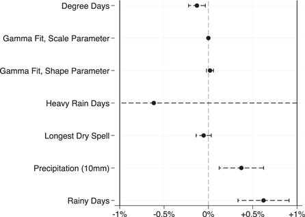
Figure 2. Estimated coefficients from a multivariate regression of (log) rice yield on heat exposure (degree days), total precipitation (including a square term), and various measures of the distribution of precipitation, as described in the main text. To facilitate comparison, the duration of the longest dry spell and the parameters of the fitted gamma distribution are normalized so that an additional rainy day increases their value by one, on average. Dashed lines indicate 95% confidence intervals. Note: the confidence interval of the coefficient of the number of heavy rain days exceed graph boundaries at (−4, 2.8).
Download figure:
Standard image High-resolution imageTo assess the suitability of a linear control of the number of rainy days in the regressions, non-parametric plots of the impact of the number of rainy days on rice yield (figure 3) are performed in two stages. First, this variable and (log) yield are both regressed on district specific intercepts, state-specific time trends and the other independent weather variables (including quadratic total precipitation and growing degree terms); second, a local polynomial (kernel) regression of the yield residual on the residual of the weather variable is estimated. The plot justifies using a linear model for the number of rainy days.
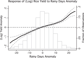
Figure 3. A non-parametric fit of rice yields on inter-annual fluctuations in the number of rainy days justifies a linear regression model. The solid curve represents a local polynomial fit (Epanechnikov kernel regressions), with 95% confidence intervals (dashed lines), of (log) yield anomaly (left axis) versus the anomaly in the number of rainy days in a given year's rainy season. Yield and rainy days anomalies are calculated as the residuals of regressions on state-specific quadratic time trends, district fixed effects, and quadratic functions of degree days and total precipitation. The root mean square anomaly sizes are 10 rainy days (n = 8523, sample mean = 85). The histograms displays the distribution of rainy days anomaly observations (fraction of observations falling in each bin, right axis).
Download figure:
Standard image High-resolution imageThe remainder of the analysis is therefore focused on the number of rainy days, and other measures of variability are omitted for simplicity. Table 1 reports the estimated regression coefficients of a log-linear model of rice yields on total rainfall, heat exposure and the number of rainy days. Coefficients are presented in terms of 0.01 logarithmic units, so that they can be approximately interpreted as the number of percentage points by which rice yield are estimated to change per unit increase in the respective weather variable. For comparison, column 1 reports estimates of a conventional model that only includes total precipitation and heat exposure. The coefficients are both statistically significant (p < 0.01) and reveal that, in agreement with previous statistical and simulation-based studies of crop yields in India [21, 35–38, 45], increases in total precipitation had a positive effect and increases in heat exposure had a negative effect on crop yields. Column 2 reports estimates of a parallel model which controls for heat exposure but replaces total precipitation with the number of rainy days. Column 3 reports estimates of a model that controls for both total precipitation and the number of rainy days simultaneously. Results reveal that for each additional rainy day, keeping heat exposure and total precipitation fixed (which amounts to a more even intra-seasonal distribution of rainfall), rice yields increase by an estimated 0.83%. In comparison, an additional 12 mm of total precipitation (the daily precipitation of an average rainy day), keeping the number of rainy days fixed, increases yield by a much smaller amount of 0.13% (0.11% × 12 mm/10 mm), half the estimate of the conventional model. Similarly, an additional degree-day reduces yields, on average, by 0.09%. A two-dimensional plot of the estimated yield response function is displayed in the right panel of figure 1. The plot illustrates the tradeoff between higher total rainfall (horizontal axis) and more uneven distributions (vertical axis) in terms of rice yields (illustrated by color).
These results are broadly maintained in a variety of alternative model specifications reported in columns 4–7 of table 1, including nonlinear temperature and precipitation controls and year fixed effects. Column 4 adds a square precipitation term. In column 5 nonlinear controls for heat exposure (dummy indicators for each interval of size 100°days in which the observation may fall) are included. In column 6 year specific dummies are added, and in column 7 additional dummies for every combination of year and state in the sample are also included. The latter two models (column 8 especially) are therefore estimated from substantially more restricted variation in weather, but the pattern of results persists. In particular, the coefficient of the number of rainy days remains highly significant and larger than that of total precipitation (which actually loses statistical significance in column 7).
The table also reports the adjusted R2 and AIC values of each model, but AIC values are reported in relation to that of a benchmark model that only controls for district specific intercepts and state specific quadratic time trends. This benchmark model has an adjusted R2 = 0.735 and AIC = 84213. High explanatory power results from the inclusion of numerous intercepts and time trends in the model. These controls are necessary in order to statistically isolate the impact of random weather fluctuations within the same location, as is widely practiced in the literature, but they mechanically explain the bulk of the variation in yields. As a result, the addition of weather controls only provides marginal improvements in explanatory power and neither measure of model quality is appropriate in this context. Nevertheless, I note that a model with rainy days outperforms a model with only total precipitation (and its square) in terms of both measures of model fit.
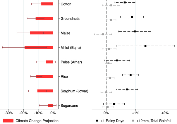
Parallel coefficient estimates for all other major rainy season crops are summarized in the right panel of figure 4. To facilitate comparability of coefficient magnitudes, the impact of total precipitation is presented in units of 12 mm, the average addition of one rainy day to total rainfall. Across all crops, the impact of an additional rainy day, keeping total rainfall fixed, is shown to be larger and more statistically significant than the effect of an average increase in total rainfall corresponding to the addition of one rainy day.
Figure 4. Estimated changes in (log) yields (horizontal axis) for major rainy season crops (vertical axis). Right panel: estimated changes in yields resulting from one additional rainy day (black squares) and total precipitation (in units of 12 mm, grey squares), from a regression of (log) yields on the number of rainy days and total precipitation,1970–2003, as described in the text. Dashed lines indicate 95% confidence intervals. Total precipitation is measured in units corresponding to the average increase in total precipitation resulting from one additional rainy day (12 mm), to facilitate comparability of the magnitude of the impacts. Left panel: projected impacts for 2050 crop yields (red bars) resulting from shifts in precipitation patterns associated with a climate change scenario based on the IPCC scenario A1B for South Asia, consisting of an increase of 100 mm in total precipitation (about 10% of the national average) and a decline of 15 rainy days (about 17% of current national average), as described in the text. Red lines indicate 95% confidence intervals.
Download figure:
Standard image High-resolution image
Illustrative simulation of climate change impacts. As a stylized illustration of the impacts of future increases in rainfall variability, regression estimates are applied to a climate change scenario for South Asia that includes a 100 mm increase in total precipitation (inspired by the IPCC's A1B, South Asia, 2080–2099 median projection of a 10% increase in precipitation) and a decrease of 15 rainy days by 2050 cited by IPCC AR4 [46, 47]. The simulation is meant to simply illustrate the importance of the precipitation distribution and does not intend to replace a full ensemble projection of 2050 impacts. Note that using the 2080–2099 projection of total precipitation increases for a 2050 impact simulation biases the projection upward (making impacts more positive), but the results reported above make it clear that this bias is small and inconsequential for the overall conclusion. Simulation results are presented in the right panel of figure 1, in which a standard projection (based on changes in heat exposure and total rainfall) and an expanded projection (which also accounts for changes in the number of rainy days) are superimposed on a two-dimensional plot of the estimated yield response function. Accounting for intra-seasonal variability flips the sign of the net projected impact due to changes in precipitation patterns, from a modest gain of 2% to a loss of 11% in 2050 rice yields relative to the counterfactual scenario of an unchanging climate, independently of the impact of increasing temperatures. Similar results are obtained for most other major rainy season crops (left panel of figure 4).
Discussion
The analysis in this paper demonstrates the importance of intra-seasonal precipitation variability for crop yields in India. Increasing variability in this distribution, as measured by the number of rainy days, is found to have had robust negative impacts on crop yields that are stronger than the positive effects of comparable increases in total precipitation. This is also illustrated by a stylized projection of the impacts of climate change on rice yields in 2050, which shows the projected impacts of variability are large enough to overturn the positive impacts of expected increases in total precipitation, shifting the net projected precipitation-driven impact from a modest positive gain to a large loss in yields (in addition to and independently of the negative impact of temperature increases). The results imply that shifts in the intra-seasonal distribution of precipitation may have important but under-studied impacts on future crop yields, and highlight the importance of projecting changes in these metrics in global climate model based studies of future climate change.
An analysis based on a statistical analysis of historical yields achieved by actual farmers is an important complement to crop-model based simulations that find substantial impacts of weather variability on yields. However, this 'reduced-form' approach, while statistically robust, is also limited in some ways. In particular, it does not allow us to narrow down the physiological mechanism underlying the observed relationships, such as the particular dominance of the number of rainy days vis a vis other measures of variability. Additional, localized studies including observations of plot-level yields in experimental farms and crop-simulation models developed for Indian agriculture are necessary in order to better understand the precise physiological processes involved and possible adaptation strategies.
Acknowledgments
I gratefully acknowledge financial support by the Harvard Sustainability Science Program during parts of this research. I thank the Columbia Water Center for their help, particularly with climate and agricultural data, obtained in part through financial support from the Pepsico Foundation.