

Abstract
The decline in Arctic sea ice cover has been widely documented and it is clear that this change is having profound impacts locally. An emerging and highly uncertain area of scientific research, however, is whether such Arctic change has a tangible effect on weather and climate at lower latitudes. Of particular societal relevance is the open question: will continued Arctic sea ice loss make mid-latitude weather more extreme? Here we analyse idealized atmospheric general circulation model simulations, using two independent models, both forced by projected Arctic sea ice loss in the late twenty-first century. We identify robust projected changes in regional temperature and precipitation extremes arising solely due to Arctic sea ice loss. The likelihood and duration of cold extremes are projected to decrease over high latitudes and over central and eastern North America, but to increase over central Asia. Hot extremes are projected to increase in frequency and duration over high latitudes. The likelihood and severity of wet extremes are projected to increase over high latitudes, the Mediterranean and central Asia; and their intensity is projected to increase over high latitudes and central and eastern Asia. The number of dry days over mid-latitude Eurasia and dry spell duration over high latitudes are both projected to decrease. There is closer model agreement for projected changes in temperature extremes than for precipitation extremes. Overall, we find that extreme weather over central and eastern North America is more sensitive to Arctic sea ice loss than over other mid-latitude regions. Our results are useful for constraining the role of Arctic sea ice loss in shifting the odds of extreme weather, but must not be viewed as deterministic projections, as they do not account for drivers other than Arctic sea ice loss.
Export citation and abstract BibTeX RIS
1. Introduction
The decline in Arctic sea ice cover has been widely documented (e.g., Stroeve et al 2012a, 2012b) and it is clear that this change is having profound impacts locally (e.g., Post et al 2013, Bhatt et al 2014). An emerging and highly uncertain area of scientific research, however, is whether such Arctic change has a tangible effect on weather and climate at lower latitudes. Of particular societal relevance is the open question: is Arctic sea ice loss making mid-latitude weather more extreme? This question has recently received a lot of scientific and media attention (see reviews by Cohen et al 2014, Vihma 2014, Walsh 2014, Barnes and Screen 2015). It has been suggested, for example, that Arctic sea ice loss may have increased the frequency of cold winters over North America and Eurasia (Liu et al 2012, Tang et al 2013, Mori et al 2014) and increased the severity of summer heatwaves (Tang et al 2014, Coumou et al 2014, 2015). Conversely, other authors have argued for fewer daily cold extremes (Screen 2014, Screen et al 2015, Schneider et al 2015).
Regardless of past changes in extremes, which may be difficult to detect or to attribute to Arctic influence (Barnes and Screen 2015), the expectation is that Arctic sea ice loss and warming will continue over the coming decades (Boe et al 2009, Mahlstein and Knutti 2012, IPCC 2013). Therefore, a logical question to ask is: will continued Arctic sea ice loss make mid-latitude weather more extreme in the future? We focus our attention on this important question.
The answer to the question posed above may depend on what is meant by 'extreme weather'. There is no single definition of what constitutes 'extreme weather'. However, the world meteorological organisation (WMO) expert team on climate change detection and indices (ETCCDI) recommends the use of twenty-seven core indices to characterize extreme weather (Zhang et al 2011). These indices, or subsets thereof, have previously been applied to observations (Alexander et al 2006, Donat et al 2013), historical climate model simulations (Sillman et al 2013a), and model projections forced by greenhouse gas increases (Sillman and Roeckner 2008, Sillman et al 2013b). These indices have also been used in the intergovernmental panel on climate change (IPCC) assessment reports (e.g., IPCC 2013).
Briefly, previous work based on projections from the fifth coupled model intercomparison project (CMIP5) multi-model ensemble has shown that increasing greenhouse gas concentrations result in a decrease in cold extremes and an increase in hot extremes (e.g., IPCC 2013, Kharin et al 2013, Sillman et al 2013b). In high latitudes, these changes are not symmetric with larger declines in cold extremes than increases in warm extremes (Kharin et al 2007, 2013), reflecting reduced temperature variance (Screen 2014). Such changes in temperature extremes are highly robust across models. Projected changes in precipitation extremes are more regionally variable. The CMIP5 models robustly project increases in precipitation extremes over high latitudes (Sillman et al 2013b). By the late twenty-first century, and if emissions are unabated, the majority of models project significantly more frequent and more severe wet (and very wet) days over the mid-latitudes, except for the Mediterranean and southern North America which are projected to become drier (Sillman et al 2013b).
Here for the first time we systemically apply a large subset (sixteen) of these indices to idealized atmospheric general circulation model (AGCM) simulations forced by projected Arctic sea ice loss, to isolate and quantify changes in temperature and precipitation extremes arising solely due to diminished Arctic sea ice cover.
2. Data and methods
2.1. Simulations
We analyse simulations from two independent AGCMs, namely, the UK Met Office Hadley centre global atmospheric model version 2 (HadGAM2) and the National Centre for Atmospheric Research (NCAR) community atmosphere model version 4 (CAM4). Full descriptions are these AGCMs can be found in Collins et al (2011) and Gent et al (2011), respectively. The version of HadGAM2 used here has a horizontal resolution of 1.875° longitude and 1.25° latitude (known as N96) and 38 vertical levels. The utilized configuration of CAM4 has a horizontal resolution of 1.25° longitude by 0.9° latitude and 26 vertical levels.
We performed two core experiments with both AGCMs. In the first experiment, we prescribed a repeating annual-cycle of sea surface temperatures (sst) and sea ice concentrations (sic) representative of the late twentieth century. These sst and sic values were taken from the CMIP5 'historical' simulations with the coupled versions of the models (known as HadGEM2 and CCSM4), averaged for the period 1980–99 and across all available ensemble members. The late twentieth century simulations with HadGAM2 and CAM4 are referred to hereafter as had20c and cam20c, respectively.
In the second experiment, we prescribed the same sst values as just described, but this time with sea ice conditions representative of the late twenty-first century. The sic values were taken from the CMIP5 'rcp8.5' simulations averaged for the period 2080–99 and across all available ensemble members. The 'rcp8.5' simulations are forced by a continuous increase in greenhouse gas concentrations and are often viewed as a 'business-as-usual' scenario, with limited mitigation strategies applied. This scenario was chosen to maximize the signal-to-noise ratio. In grid-boxes that lost ice between the late twentieth and twenty-first centuries, the sst value for the late twenty-first century was used. This procedure accounts for the ocean surface warming in regions where ice is reduced. The late twenty-first century simulations with HadGAM2 and CAM4 are referred to hereafter as had21c and cam21c, respectively. Further details on the experimental setup can be found in Screen et al (2015). Additionally in the supplementary material, we present selected results from a third experiment with mid-twenty-first century sea ice conditions (had21c_mid and cam21c_mid).
The mean March (month of annual maximum) and September (month of annual minimum) sea ice concentrations, and the annual cycle of Arctic sea ice area, from each simulation are shown in figure 1. In September there are ice-free conditions in both had21c and cam21c. In fact, had21c is ice-free (or very nearly) from July to November and cam21c is ice-free from August to October. In March, had21c retains ice along the northern coasts of Greenland, Canada and Siberia, but open water dominates the Atlantic sector. In comparison, cam21c retains more multi-year ice with the largest reductions (compared to cam20c) in the Barents Sea, Sea of Okhotsk and Bering Sea. In terms of mean March sea ice area, had21c has a 50% reduction (compared to had20c) and cam21c has a 20% reduction (compared to cam20c). The CMIP5-mean loss of March sea ice area over this time period (under rcp8.5) is 32% (15%–63%; 5th–95th percentile range). Thus, the prescribed sea ice area loss in HadGAM2 is towards the upper-end of the CMIP5 model spread and in CAM4, is towards the lower end.
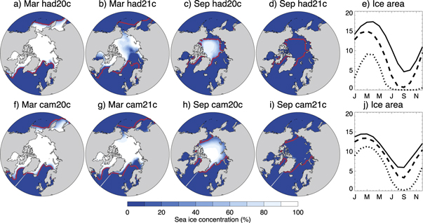
Figure 1. March sea ice concentrations in (a) had20c and (b) had21c and September sea ice concentrations in (c) had20c and (d) had21c. (e) Annual cycle of Arctic sea ice area (106 km2) in had20c (solid curve), had21c (dotted curve) and had21c_mid (dashed curve). March sea ice concentrations in (f) cam20c and (g) cam21c and September sea ice concentrations in (h) cam20c and (i) cam21c. (j) Annual cycle of Arctic sea ice area (106 km2) in cam20c (solid curve) and cam21c (dotted curve) and cam21c_mid (dashed curve). Magenta contours show the sea ice extent (defined as the 15% contour) in (a)–(d) had20c and (f)–(i) cam20c.
Download figure:
Standard image High-resolution imageAll simulations (had20c, cam20c, had21c and cam21c) were run for 260 years. In our modelling framework where the boundary forcing repeats annually, each year can be considered a separate ensemble member starting from a different atmospheric initial condition. Thus, we have 260-member ensembles from which to calculate robust statistics of extreme weather. We note that since these are atmosphere-only simulations, we cannot capture possible changes in weather extremes related to ocean circulation changes that may result from Arctic sea ice loss (Deser et al 2015).
In what follows we analyse daily values of maximum near-surface (1.5 m in HadGAM2; 2 m in CAM4) temperature (Tmax), minimum near-surface temperature (Tmin), daily-mean near-surface temperature (Tave) and total precipitation (Ptot). We applied the ETCCDI indices (see below) to the full 260 years and then derived long-term means. To approximate the response to Arctic sea ice loss, we subtracted the long-term mean of the had20c (cam20c) simulation from that in the had21c (cam21c) simulation. Statistical significance was calculated using a difference of means test (Student's T-test) where the null hypothesis is that the two samples (n = 260) have the same mean. We report responses where the null hypothesis can be rejected with 95% confidence. In addition to testing for statistical significance, we also assess the robustness of the response between the two models. Robust responses are considered to be those for which there is model agreement on the sign and significance (i.e., the response is significant at the 95% confidence level in both models).
2.2. Extreme indices
We analyse sixteen of the ETCCDI core indices, which are only briefly introduced here; full definitions can be in Zhang et al (2011). Specifically these are (official identifier in parentheses): frost days (FD; annual count of days when Tmin < 0 °C), icing days (ID; annual count of days when Tmax < 0 °C), cold nights (TN10p; % of days when Tmin < 10th percentile), cold days (TX10p; % of days when Tmax < 10th percentile), cold spell duration (CSDI; annual count of days with at least 6 consecutive days when Tmin < 10th percentile), warm nights (TN90p; % of days when Tmin > 90th percentile), warm days (TX90p; % of days when Tmax > 90th percentile), warm spell duration (WSDI; annual count of days with at least 6 consecutive days when Tmax > 90th percentile), wet days (R10mm; annual count of days when Ptot > = 10 mm), very wet days (R20mm; annual count of days when Ptot > = 20 mm), wet day precipitation (R95pTOT; annual total precipitation on days when Ptot > 95th percentile), very wet day precipitation (R99pTOT; annual total precipitation on days when Ptot > 99th percentile), precipitation intensity (SDII; average precipitation on days when Ptot > = 1 mm), longest wet spell (CWD; annual maximum number of consecutive days when Ptot > = 1 mm), dry days (Rnnmm; annual count of days when Ptot = 0 mm; see note below) and longest dry spell (CDD; annual maximum number of consecutive days when Ptot < 1 mm). We note that one ETCCDI index is user-defined (Rnnmm; annual count of days when Ptot is above a user-chosen threshold); here we apply a threshold of 0 mm and refer to this index as dry days. For the percentile-based indices, the percentile thresholds were determined from the late twentieth century simulations (had20c and cam20c) and kept the same for the evaluations of the changes in these indices in the late twenty-first century.
The indices were calculated at each model grid-point before regional averaging, using twelve regional domains (shown in figure 3(a)) based on those defined in the IPCC special report on managing the risks of extreme events and disasters to advance climate change adaptation (SREX; Seneviratne et al 2012) and later used in the IPCC fifth assessment report (IPCC 2013). These are: Alaska and western Canada (AWC; 105–168 °W 50–75 °N), eastern Canada and Greenland (ECG; 10–105 °W 50–85 °N), Scandinavia (SCA; 0–40 °E 58–85 °N), Siberia (SIB; 40–180 °E 50–85 °N), western United States (WUS; 105–130 °W 30–50 °N), central US (CUS; 85–105 °W 30–50 °N), eastern US (EUS; 60–85 °W 30–50 °N), central Europe (CEU; 10 °W–40 °E 45–58 °N), Mediterranean (MED; 10 °W–40 °E 30–45 °N, western Asia (WAS; 40–75 °E 30–50 °N), central Asia (CAS; 75–100 °E 30–50 °N) and eastern Asia (EAS; 100–145 °E 30–50 °N). We hereafter refer to these regions by the three letter abbreviations just provided.
2.3. Model evaluation
To evaluate the models' ability to simulate realistic weather extremes, we compared climatological values of the ETCCDI indices (for the non-percentile-based indices) in the late twentieth century simulations to estimates of these quantities in the real world. Since there is large observational uncertainty, we utilize four different reference data sets: HadEX2 (Donat et al 2013), based solely on in situ observations, and three commonly used reanalysis products, ERA-Interim (Dee et al 2011), NCEP/DOE (Kanamitsu et al 2002) and NCEP/NCAR (Kalnay et al 1996). The two models simulate well the main spatial features of the observed climatologies of the ETCCDI indices (supplementary figure 1), for example, the latitude and altitude dependence of cold extremes and enhanced precipitation extremes in coastal and mountainous regions. Figure 2 shows the mean biases in the models, compared to each reference data set, averaged within our regional domains. More specifically, we area-averaged each index over our twelve regions and compared the regional averages derived from had20c and cam20c to those from the reference data sets. The biases were simply calculated by subtracting the reference value (area and time mean) from the simulated value, such that a positive bias implies the model, on average (in space and time), overestimates the quantity of interest. For most indices and regions, the magnitudes of the biases vary considerably depending on the reference data set used (in some cases the biases are of opposite sign). This prevents a meaningful quantitative assessment of the model biases; however, there are some consistent features of the biases (corroborated by multiple reference data sets) that enable qualitative statements on the ability of the models to simulate particular types, or characteristics, of extreme weather. The models have generally smaller biases for the 'event frequency' indices, for example frost days or wet days (R10mm), than for the 'event duration' indices. Most notably, both models substantially overestimate the mean cold spell duration (CSDI). They also tend to underestimate dry spell duration (CDD), but these biases are smaller than for cold spells. Relatively large biases are also identified for warm spell duration (WSDI), but the sign of these vary between the reference data sets, complicating their interpretation. Given the large observational uncertainty, biases in all the indices likely reflect inadequacies in the observations as well as in the models.
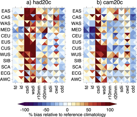
Figure 2. Mean biases in (a) had20c and (b) cam20c relative to observed estimates, expressed as percentages of the reference climatological values. Biases are calculated for 9 ETCCDI indices (x axes) each averaged over the twelve regions (y axes). For each index and region, the coloured quadrants show biases calculated relative to four different reference data sets: HadEX2 (top), ERA-Interim (right), NCEP-NCAR (bottom) and NCEP-DOE (left). The reference climatologies are based on the 1981–2010 period (except for HadEX2, which uses 1961–1990). Grey shading indicates insufficient reference data (defined here as >20% of grid-boxes within the regional domain with <30 years of data).
Download figure:
Standard image High-resolution imageSillman et al (2013b) assessed the ability of the CMIP5 models (including HadGEM2-ES and CCSM4) to simulate observed global climatologies of the ETCCDI indices. HadGEM2-ES and CCSM4 were shown to perform comparatively well in this regard with generally small biases globally (see their figure 10), and to out-perform most other CMIP5 models (especially for the precipitation indices). Thus despite the substantial biases shown in figure 2, we consider these models to be two of the best available for studying future changes in extremes in response to sea ice loss. However, the projected changes in the ETCCDI indices arising from sea ice loss revealed in the following sections need to be viewed with a degree of caution in light of the model climatological biases in these indices.
3. Results
3.1. Cold extremes
Both models project significant reductions in frost days (figure 3(b)), icing days (figure 3(c)), cold nights (figure 3(d)) and cold days (figure 3(e)) over the high-latitude regions; namely, AWC, ECG, SCA and SIB. Both models also project significantly fewer frost days, icing days, and cold nights over certain mid-latitude regions; namely, CUS and EUS. Also, cold days decrease in both models over EUS and a small, but statistically significant, reduction in frost days is projected over MED. CAS is the only region for which both models project an increase in any of the aforementioned indices, a small, but significant, increase in cold nights. Projected changes in these indices over WUS, CEU, WAS and EAS are either statistically insignificant in one or both of the models, or are of opposite sign in the two models and thus, cannot be considered to be robust. Regarding the latter, frost days and icing days over WAS both decrease in HadGAM2 but increase in CAM4, and cold nights and cold days over WUS both increase in HadGAM2 but decrease in CAM4.
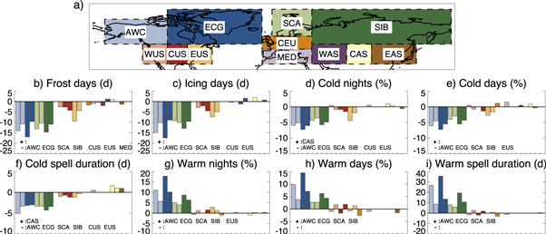
Figure 3. Projected changes in regional temperature extremes in response to Arctic sea ice loss. Each bar graph (b)–(i) corresponds to a different extreme index. Within each bar graph the pairs of coloured bars correspond to averages over the coloured regions in the map (a), and in each pair the left and right bars correspond to HadGAM2 and CAM4, respectively. Bars are only shown for responses that are statistically significant at the 95% confidence level. Robust regional responses (i.e., models agree on the sign and significance of the response) are listed at the bottom of each graph. Note that the vertical axes have different units (provided in each sub-title) and scales.
Download figure:
Standard image High-resolution imageAs well as altering the frequency of cold extremes, Arctic sea ice loss may effect the duration of cold extremes. Indeed, a shift towards more prolonged cold extremes has been hypothesized (Francis and Vavrus 2012, 2015). Turning then to cold spell duration (figure 3(f)), both models project significant decreases over AWC, ECG, SCA, SIB, CUS and EUS, but a significant increase over CAS. The shift towards shorter cold spells, especially over the central and eastern US, is opposite to that hypothesized by some in response to Arctic warming.
In summary, both models depict the largest reduction in cold extremes and their duration over the high latitudes. Over mid-latitudes, there are consistent reductions in cold extremes and their duration over central and eastern US, but little change over Europe. Central Asia is unique in being the only region where cold extremes are projected to increase in frequency and length.
3.2. Hot extremes
Both models depict significant increases in warm days (figure 3(g)) and warm nights (figure 3(h)) over the high latitude regions of AWC, ECG, SCA and SIB. Also, warm nights increase significantly over EUS in both models. In general over mid-latitudes, the changes in warm extremes are less robust than those in cold extremes. For example over WUS, HadGEM2 projects significant decreases in warm nights and warm days, whereas both indices significantly increase in CAM4. Similar model divergence is found for warm nights over CAS and warm days over CUS and EUS.
Next we consider warm spell duration (figure 3(i)), which like cold spell duration, has also been hypothesized to increase in response to Arctic warming (Tang et al 2014, Coumou et al 2015). Warm spells are projected to lengthen over AWC, ECG, SCA and SIB in both models in response to Arctic sea ice loss. However, no robust changes in this index are projected over the mid-latitudes.
In summary, robust increases in warm extremes and their duration are projected over the high-latitudes, but the mid-latitude changes are weak and non robust.
3.3. Wet extremes
Significant increases in wet days (figure 4(b)) and in very wet days (figure 4(c)) are projected by HadGAM2 for all regions considered. Fewer of the regional changes are significant in CAM4, but those that are, are predominantly positive. CAM4 depicts significant increases in wet days over AWC, ECG, SIB, MED and CAS; and very wet days over the same regions (except AWC, where the change is insignificant). In contrast to HadGAM2, CAM4 projects a significant decrease in wet days and very wet days over CUS, and in wet days over SCA.

Figure 4. Projected changes in regional precipitation extremes in response to Arctic sea ice loss. The bar graphs are analogous to those in figure 2, but for indices of precipitation extremes.
Download figure:
Standard image High-resolution imageTotal wet day precipitation (figure 4(d)) and total very wet day precipitation (figure 4(e)) also increase significantly across the majority of regions in HadGEM2. Again the changes in these indices are weaker in CAM4. CAM4 projects significant increases in one or both these indices over ECG, SIB, MED and CAS; but a decrease in the former index over CUS.
The precipitation intensity index (figure 4(f)) documents changes in the average amount of precipitation on wet days. Thus, this metric is a measure of the severity of wet extremes rather than their frequency. Precipitation intensity increases significantly in all regions in HadGAM2. Significant changes are also projected in some regions in CAM4, but they are of mixed sign. Precipitation intensity increases significantly over CAS, but decreases significantly over AWC, SCA, SIB, EUS and EAS.
Next, the longest wet spell index (figure 4(g)) provides a measure of the annual average maximum duration of wet spells. The longest wet spell increases significantly in HadGAM2 for all regions except SCA. In CAM4, this index increases significantly for five of the twelve regions, specifically, AWC, ECG, SIB, CAS and WAS; and decreases significantly for CEU. The latter change mirrors decreases in wet day (and very wet day) precipitation and precipitation intensity over this region in CAM4, but is in stark contrast to the increases projected by HadGAM2.
In summary, the two models project contrasting changes in wet extremes. HadGAM2 depicts significant increases in the frequency, severity and duration of wet extremes over all or most regions. In contrast, the changes in CAM4 are of mixed sign and significance.
3.4. Dry extremes
Dry days (figure 4(h)), i.e. days with no precipitation, are generally projected to decrease, especially over mid-latitude Europe and Asia. Both models depict significant reductions in dry days over SIB, EUS, CEU, WAS, CAS and EAS. The models diverge significantly over ECG (HadGAM2 increases; CAM4 decreases) and CUS (HadGAM2 decreases; CAM4 increases).
Lastly, the longest dry spell (figure 4(i)) is projected by HadGAM2 to decrease in all regions, except SCA. Significant decreases are corroborated by CAM4 over AWC, ECG, SIB and EAS. The only region with a significant increase in dry spell length, in either model, is SCA in HadGAM2.
In summary, there is an overall tendency for fewer dry days and shorter dry spells in both models, although these changes are significant over more regions in HadGAM2 than they are in CAM4.
4. Discussion
The regions with projected reductions in cold extremes coincide with regions of annual-mean warming (figure 5(a)). The loss of sea ice induces local warming (Screen et al 2012, 2013, 2014), which is advected to neighbouring regions by the mean atmospheric circulation and transient eddies (Deser et al 2010), causing mean warming in mid-latitudes. Accompanying this mean warming is a decrease in high- and mid-latitude daily temperature variance (figure 5(b)), arising from the reduced north-south temperature gradient (Screen 2014, Schneider et al 2015, Screen et al 2015). Both the mean warming and reduced variance favour fewer cold extremes. It is notable that the warming and reduced variance are of larger magnitude over EUS than for any of the other mid-latitude regions (figure 5). The mean tropospheric circulation over North America, which displays a southward dip east of the Rocky Mountains, appears conducive for propagating the Arctic warming signal to mid-latitudes over central and especially, eastern North America compared to other mid-latitude regions. Also, reductions in Hudson Bay sea ice, which occur at relatively low latitudes compared to other longitudes, may enhance the response over eastern North America. Hence, the decline in cold extremes is more pronounced and robust here than in other mid-latitude regions.
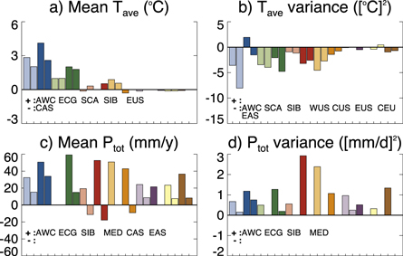
Figure 5. Projected changes in annual-mean temperature (a), daily temperature variance (b), annual total precipitation (c) and daily precipitation variance (d) in response to Arctic sea ice loss. The bar graphs are analogous to those in figure 2.
Download figure:
Standard image High-resolution imageThe CAS region is unique in displaying a robust cooling response (figure 5), which helps explain the robust increase in cold nights and cold spell duration for this region only (figure 3). The cooling response appears to be dynamically driven and associated with a strengthened Siberian High (supplementary figure 2), which enhances cold air advection to the region, consistent with previous work (e.g., Mori et al 2014, Screen et al 2015).
The increase in hot extremes over high latitudes (figure 3) is consistent with the overall warming response (figure 5). Over mid-latitudes, where mean temperature changes are weaker and less robust (figure 5), the changes in hot extremes are also weaker and less robust (figure 3). The robust reductions in variance over many mid-latitude regions do not all coincide with fewer hot extremes (although there are some such cases, e.g., for WUS, CUS and CEU in HadGAM2 where warm days and warm spell duration decrease). This is consistent with the interpretation that projected variance reductions primarily arise due to warming at the cold (left-hand) tail of the temperature distribution (Screen 2014).
The projected changes in temperature extremes in response to sea ice loss by the mid-twenty-first century are, in general, of the same sign as those found for the late twenty-first century, but with reduced magnitude and statistical significance (supplementary figure 3). The mid-century robust responses are largely confined to the high-latitude regions, although robust decreases in icing days and increases in warm nights are projected for EUS.
Turning now to the projected precipitation response to late twenty-first century sea ice loss, the regions with robust increases in the frequency of precipitation extremes (i.e., wet days or very wet days) all show robust increases in both mean annual total precipitation and daily precipitation variance (figures 5(c) and (d)).
The model divergence between the projected changes in precipitation extremes—specifically, the larger and more spatially coherent changes in HadGAM2 than in CAM4—warrants further exploration and explanation. On closer inspection, the changes in the annual precipitation extreme indices arise predominantly from large increases in summer extremes in HadGAM2 (e.g., monthly responses of maximum 1-day and 5-day precipitation [rx1day, rx5day] peak in summer in all regions; not shown). In turn, the differences in extreme precipitation responses can be traced to differences in the annual cycle of the mean precipitation response in the two models, predominantly over land regions. Whilst both models depict a broadly consistent annual cycle of precipitation response over the high-latitude ocean (a maximum in fall/winter and minimum in summer; albeit with differing magnitude owning to larger sea ice losses in HadGAM2 than in CAM4), they depict contrasting annual cycles over the high-latitude land regions (figure 6). Here, CAM4 shows small changes that peak in the fall and winter, whereas HadGAM2 shows a large peak in late spring and early summer. This summer maximum is also projected over the mid-latitude landmasses in HadGAM2, whereas in CAM4 there is little seasonality in the response.
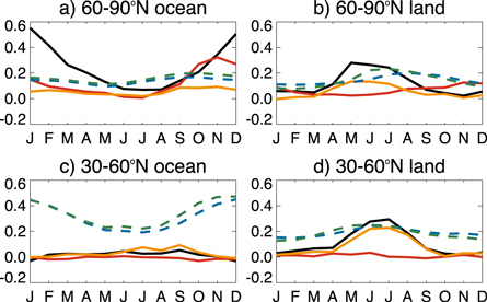
Figure 6. Annual cycle of the monthly-mean precipitation (mm d–1) response to Arctic sea ice loss averaged over the (a) high-latitude ocean, (b) high-latitude land, (c) mid-latitude ocean and (d) mid-latitude land. The black and red lines show projected responses from HadGAM2 and CAM4, respectively. The orange lines show the responses in HadGAM2 mid-twenty-first century experiment. The dashed green and blue lines show the climatological annual cycle of precipitation in had20c and cam20c, respectively (note these climatological values have been divided by a factor of 10 so that they plot on the same vertical axis as the responses).
Download figure:
Standard image High-resolution imageOne possible explanation for the varied seasonal precipitation responses in the two models is the differing sea ice forcing: recall, had21c has considerably more open water in summer than cam21c. However, an additional experiment using HadGAM2 but with mid-twenty-first century sea ice conditions (had21c_mid), in which the summer sea ice area closely matches that in cam21c (figure 1), also projects a marked increase in summer land precipitation relative to had20c (figure 6; orange lines) and annual precipitation extremes (supplementary figure 4). Therefore, it appears that the enhanced summer land precipitation response in HadGAM2 compared to CAM4 is not primarily due to differences in sea ice forcing between the models. We further note that the two models have very similar climatological annual cycles of precipitation (figure 6; dashed lines) and hence, the differences in forced response do not appear to arise because of differences in mean precipitation.
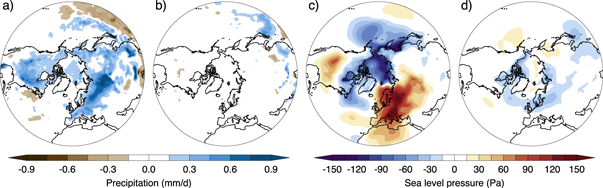
Spatial maps of the summer precipitation and sea level pressure (SLP) responses provide additional insight into the causes of the differing summer precipitation responses in the two models. As mentioned above, the summer precipitation increase in HadGAM2 is enhanced over land regions and, as revealed in figure 7(a), especially over Eurasia. This local intensification of the precipitation response may partly arise from the circulation response, with HadGAM2 projecting an anomalous anticyclone over Eurasia (figure 7(c)). Also, a precipitation response dipole over the western Pacific is co-located with a SLP dipole. None of these features are identifiable in the CAM4 precipitation (figure 7(b)) or SLP (figure 7(d)) responses. Thus, model differences in the atmospheric circulation response likely contribute to the differing precipitation responses in the two models. However, it is unclear whether the circulation changes can fully explain the ubiquitous summer precipitation increase over land in HadGAM2. It is possible that land-surface feedbacks and/or convective processes may also play a role, and that the differing summer precipitation responses in the two models may further reflect differing model representation of these processes.
Figure 7. Projected changes in summer (June–July–August) precipitation (a), (b) and sea level pressure (c), (d) in response to Arctic sea ice loss. Projected responses from HadGAM2 are shown in (a) and (c), and from CAM4 in (b) and (d).
Download figure:
Standard image High-resolution image
5. Conclusions
We have applied the ETCCDI extreme indices to simulations from two independent AGCMs, both forced solely by projected Arctic sea ice loss in the late twenty-first century. On the basis of these model simulations and considering only those projected changes that are robust (i.e., models agree on the sign and significance of the response), we conclude that future Arctic sea ice loss is most likely to:
- (1)Decrease the likelihood and duration of cold extremes over high latitudes and over central and eastern United States, but increase the likelihood and duration of cold extremes over central Asia.
- (2)Increase the likelihood and duration of hot extremes over high latitudes.
- (3)Increase the likelihood and severity of wet extremes over high latitudes (excluding Scandinavia), the Mediterranean and central Asia, and increase their duration over high latitudes, central and eastern Asia.
- (4)Decrease the likelihood of dry days over mid-latitude Eurasia and reduce dry spell duration over high latitudes.
The projected changes in temperature extremes are largest over the high latitudes, consistent with a larger mean climate response (e.g., Screen et al 2014). Considering the heavily populated mid-latitudes, where changes in extreme weather may have significant societal implications, the largest sea ice induced changes in temperature extremes are found over central and eastern North America. Here, Arctic sea ice loss appears to be an important driver of future change in hot and cold extremes. Sea ice loss reduces the likelihood of North American cold extremes, consistent with Screen et al (2015), but contrary to recent speculation (e.g., see discussion in Wallace et al 2014). We found no clear change in temperature extremes over Europe in response to sea ice loss and only very small changes over mid-latitude Asia. Our results suggest therefore, that Arctic sea ice loss is unlikely to be a major driver of future changes in temperature extremes over these regions. With regards to precipitation extremes, the regions most affected appear model dependent, based on the analysis of the two models used here. Coordinated experiments with a greater diversity of models would be valuable for assessing the robustness of future changes in precipitation extremes arising from sea ice loss.
Lastly, it is important to emphasize that we have only considered the changing risk of extreme weather due to projected Arctic sea ice loss. In reality, many other factors will influence the future climate and associated extreme weather. Our results are useful for constraining the role of Arctic sea ice loss in shifting the odds of extreme weather, but must not be viewed as deterministic projections (i.e., our best guess of the changes that will ultimately occur). For example, related to point (1) above, whilst Arctic sea ice loss may increase the odds of cold extremes over central Asia, the net effect of increasing greenhouse gas concentrations is to reduce the frequency of cold extremes (Mori et al 2014).
Acknowledgments
We thank Robert Tomas for conducting some of the CAM4 simulations. The HadGAM2 simulations were performed on the ARCHER UK National Supercomputing Service. James Screen is supported by National Environmental Research Council grant NE/J019585/1. The National Science Foundation (NSF) Office of Polar Programs supported Lantao Sun. The NSF sponsors NCAR. Two anonymous reviewers are thanked for their time and expert feedback.