

Abstract
The atmospheric levels of human-produced chlorocarbons and bromocarbons are projected to make only small contributions to ozone depletion by 2100. Increases in carbon dioxide (CO2) and nitrous oxide (N2O) will become increasingly important in determining the future of the ozone layer. N2O increases lead to increased production of nitrogen oxides (NOx), contributing to ozone depletion. CO2 increases cool the stratosphere and affect ozone levels in several ways. Cooling decreases the rate of many photochemical reactions, thus slowing ozone loss rates. Cooling also increases the chemical destruction of nitrogen oxides, thereby moderating the effect of increased N2O on ozone depletion. The stratospheric ozone level projected for the end of this century therefore depends on future emissions of both CO2 and N2O. We use a two-dimensional chemical transport model to explore a wide range of values for the boundary conditions for CO2 and N2O, and find that all of the current scenarios for growth of greenhouse gases project the global average ozone to be larger in 2100 than in 1960.
Export citation and abstract BibTeX RIS

Content from this work may be used under the terms of the Creative Commons Attribution 3.0 licence. Any further distribution of this work must maintain attribution to the author(s) and the title of the work, journal citation and DOI.
1. Introduction
Anthropogenic ozone-depleting chlorocarbons and bromocarbons are declining due to cessation of their production as a result of the Montreal Protocol and its amendments (Andersen and Sarma 2002). By the year 2100 the role of chlorine and bromine in determining the amount of ozone in the stratosphere will be small, and factors including other trace gases will control the ozone concentration.
One factor that will impact future ozone is the concentration of nitrous oxide (N2O). Reaction of N2O with excited atomic oxygen (O1D) is the primary natural source of nitrogen oxides (NOx = NO + NO2) to the stratosphere (McElroy and McConnell 1971). As NOx make the largest contribution to stratospheric ozone loss, even for elevated chlorine levels (e.g., figure 9.2 of Holloway and Wayne 2010), an increase in N2O could decrease stratospheric ozone. In fact, Ravishankara et al (2009) have shown that N2O is the dominant ozone depleting substance (ODS) currently emitted, and is expected to remain so through the remainder of the 21st century. Kanter et al (2013) have suggested that the ozone impact of N2O could be used as a basis for international regulations to control its future emissions to the atmosphere.
Another important factor that will impact future ozone levels is the concentration of carbon dioxide (CO2). CO2 cools the stratosphere, slowing temperature-dependent ozone loss processes, resulting in rising ozone levels (Brasseur and Hitchman 1988). Model calculations indicate that past and future increases in CO2 should speed-up the Brewer–Dobson circulation (e.g., Butchart et al 2006), which would decrease ozone in the tropics and increase ozone in middle and high latitudes (e.g., Austin and Wilson 2006, Shepherd 2008, Li et al 2009). The combination of cooling and the speed-up of the Brewer–Dobson circulation can lead to a 'super-recovery' of ozone at middle and high latitudes to amounts greater than observed in the pre-CFC era (pre-1960).
Cooling also affects ozone loss through its impact on the amount of nitrogen oxides. The NOx loss reaction (N + NO → N2 + O) competes with the reaction of N atoms with O2 to form NO. The N + O2 reaction is strongly temperature dependent (Sander et al 2010). Cooler temperatures favor the loss reaction, thus reducing the effectiveness of N2O in producing NOx. This feedback between temperature and NOx concentrations affects the impact of increased N2O on stratospheric ozone. For example, Rosenfield and Douglass (1998) explored the relationship between NOx and stratospheric cooling, noting that for fixed N2O boundary conditions the upper stratospheric NOx decreased by 15% for doubled CO2.
In recent years, several studies have examined the interactions of changing CO2 and N2O on ozone using two-dimensional (Fleming et al 2011, Portmann et al 2012) or three-dimensional (Oman et al 2010, Plumber et al 2010, Revell et al 2012a, 2012b, Wang et al 2014) models. These model studies have shown that CO2-induced stratospheric cooling and strengthening of the meridional circulation reduces the yield of NOx from N2O, and mitigate the effectiveness of N2O in depleting ozone. Further, for the GHG scenarios considered, changes in NOx have only a small effect on the future evolution of ozone (e.g., Oman et al 2010, Plummer et al 2010).
The above studies have focused primarily on ozone changes for a single scenario for future GHG concentrations or have examined only a limited range of N2O and CO2 boundary conditions. Here we examine the coupled impacts of changes in N2O and CO2 on stratospheric NOx and ozone for a wide range of future boundary conditions, encompassing the range of values in the year 2100 from the Intergovernmental Panel on Climate Change (IPCC) scenarios. For all of the current scenarios for growth of N2O and CO2, the model indicates larger global average column ozone in 2100 than in 1960.
2. Model and simulations
We examine the output from steady-state simulations of stratospheric composition obtained using the two-dimensional Goddard Space Flight Center coupled chemistry–radiation–dynamics model (GSFC2D). Fleming et al (2011) describe in detail this model and its performance compared with the three-dimensional Goddard Earth Observing System Chemistry Climate Model (GEOSCCM) (Pawson et al 2008). Briefly, we used the model with a 2 km vertical resolution and 10° latitude resolution. Many of the components of the GSFC2D model are the same as those in GEOSCCM. These include: the infrared (IR) radiative transfer scheme (Chou et al 2001); the photolytic calculations (Anderson and Lloyd 1990, Jackman et al 1996); and the microphysical model for polar stratospheric cloud formation (Considine et al 1994).
The dynamics in GSFC2D are coupled to chemistry through the IR heating and UV absorption. Mixing and momentum deposition are computed using a linearized parameterization. The lower boundary condition for the dynamics is solved for planetary zonal wave numbers 1–4 (see Fleming et al 2011 for details). The model includes mixing under the assumption that horizontal eddy mixing is directed along the zonal mean isentropes, and projects the Kyy mixing rates onto isentropic surfaces. The model also includes parameterized gravity wave breaking that is interactive with the mean flow (Appendix A of Fleming et al 2011).
Fleming et al (2011) show that the time-dependent ozone responses from GSFC2D and GEOSCCM models are similar for the reference simulation of ODSs and greenhouse gases used in the second phase of the SPARC validation activity for chemistry climate models (CCMVal-2) (SPARC CCMVal 2010). Additional simulations with GSFC2D (Fleming et al 2011) exploit its computational efficiency while separating the contributions of the ODSs and other time-varying source gases to ozone response. GSFC2D also produced results consistent with the GEOSCCM in 'world avoided' simulations with unabated increases in anthropogenic chlorocarbons and bromocarbons (Newman et al 2009) demonstrating that the responses of both models to large perturbations are consistent. Here we again exploit the computational efficiency of GSFC2D, this time focusing on the relative and combined effects of N2O and CO2 on both the radiation and chemistry of the stratosphere.
We examine the sensitivity of both the global amount of total reactive nitrogen (NOx plus reservoir gases NOy = N + NOx + HNO3 + ClONO2 + BrONO2) and ozone (O3) by running the GSFC2D model to a steady state for three values of the lower boundary condition for N2O (280, 360 and 440 ppbv) for each of five values of the lower boundary condition for CO2 (280, 420, 560, 700 and 840 ppmv). The units for the boundary conditions are parts per billion by volume (1 ppbv = 10−9 moles/mole) and parts per million by volume (1 ppmv = 10−6 moles/mole). For each of these simulations, CFC boundary conditions are set to achieve 2 ppbv of Cly in the upper stratosphere. This is approximately the amount experienced in 1980 and expected to be reached in 2050. The CH4 boundary condition is also set at a fixed value (1.8 ppmv) in all simulations.
3. Reactive nitrogen (NOy)
We first examine how NOy varies with N2O and CO2 boundary conditions. We focus on the globally average total column NOy ('global NOy' for short), as a simple metric for the NOy. Figure 1 presents the global NOy from the GSFC2D simulations as a function of the N2O and CO2 boundary conditions.
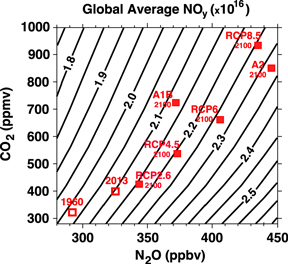
Figure 1. Global area-weighted average NOy column (in 1016 molecules/cm2) as a function of the N2O and CO2 lower boundary conditions assumed in the GSFC 2D model. In all simulations the boundary conditions for chlorine containing species sums to 2 ppbv chlorine, and the boundary condition for methane is held at 1.8 ppmv. Open red squares indicate the model results for 1960 and 2013 conditions. Filled red squares indicate the results for the year 2100 conditions for the SRES and RCP scenarios.
Download figure:
Standard image High-resolution imageFigure 1 shows that the global-average NOy increases with increasing N2O and fixed CO2. The increase in global NOy is with a near linear function of lower boundary N2O, but the relative rate of increase of NOy is less than that of N2O. For example, there is a 60% increase in N2O for the range shown in figure 1 (280–450 ppbv) but the increase in NOy is only around 32% (e.g., 2.0–2.65 ppbv when CO2 = 300 ppmv). This difference in relative increase is because N2O is not the only source of atmospheric NOy. Galactic cosmic rays, lightning, and pollution are also sources of NOy. These are included in GSFC2D and contribute about a 1/3 of the global NOy in the model at 320 ppbv N2O.
For increasing CO2 with fixed N2O boundary conditions global NOy decreases as shown in figure 1. This occurs primarily because increasing CO2 cools the stratosphere, altering the rate of chemical reactions of the production and loss of NOy. Increasing CO2 also speeds up the mean meridional circulation (so called 'Brewer–Dobson circulation') in the model, but this has less net impact on NOy. The acceleration of the Brewer–Dobson circulation pushes N2O upward in the tropics, raising the altitude at which N2O reacts with O(1D) to produce NOy and also pushing more NOy upward into the destruction region (Rosenfield and Douglass 1998).
To better understand the impact of increases in CO2 on NOy, we examine the production and loss of NOy. NOy is produced mainly from N2O via the reaction

while the NOy loss rate is controlled by the reaction

The N atoms participating in reaction (2) are generated by the photolysis of NO to form N + O. The N atoms have two possible paths; they can react with NO as in reaction (2) to reform N2 or they can react with O2 to reform NO with no net loss of NOy. Presuming steady state for nitrogen atoms, the following expression is obtained for NOy loss:
where square brackets indicate concentrations in molecules/cm3, kN,NO is the rate coefficient for the reaction of N with NO, kN,O2 is the rate coefficient for the reaction of N with O2, and JNO is the photolysis rate of NO. As the temperature decreases due to the addition of CO2 and other GHGs the rate coefficient kN,O2 decreases, reducing the denominator in equation (3) and increasing the total loss rate for NOy. Although JNO values are shown to vary widely among the CCMs that participated in CCMVal-2, differences in JNO would affect the magnitude of the loss of NOy in a given CCM but not the sensitivity of loss to cooling. The relative magnitude of the two terms in the denominator is a function of both the temperature and the amount of NO. At 10 parts per billion by volume (ppbv) of NO and 240 K the N + O2 term is about 4 times larger than the N + NO term. Thus the change in rate of the N + O2 reaction caused by cooling almost linearly translates into a change in the loss rate for NOy. Another way of thinking of this result is that a decrease in temperature favors the reaction branch of N + NO, leading to increased NOy loss due to this reaction.
To illustrate this, figure 2 shows the variation of the globally-averaged production, loss, and concentration of NOy for CO2 increasing from 300 to 850 ppmv (with N2O boundary condition fixed at 360 ppmv). As CO2 increases there is a moderate change in the NOy production but a large increase in its loss, leading to a reduction in the overall NOy concentration.
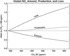
Figure 2. Variation of global-averaged loss, production, and concentration ('amount') of NOy as a function of the CO2 lower boundary condition (BC), Results assume a constant N2O (=360 ppbv) lower boundary condition. The loss term is determined from equation (3) and is not linear in the total NOy amount.
Download figure:
Standard image High-resolution imageAs increasing N2O causes global NOy to increase but increasing CO2 affects global NOy in the opposite sense, the change in global NOy when both N2O and CO2 increase depends on their relative increases. As shown in figure 1, for larger increases in CO2 relative to N2O there is a decrease in global-average NOy, whereas there is an increase in global-average NOy if the relative increase in N2O is larger.
We now consider the changes in NOy for changes in N2O and CO2 corresponding to the different Special Report on Emissions Scenarios (SRES) (IPCC 2000) or Representative Concentration Pathways (RCPs) (Moss et al 2010, Meinshausen et al 2011). The red squares in figure 3 show the increases in CO2 and N2O following different future scenarios. The open red square in figure 1 is placed at the observed N2O and CO2 values in 1960, while the filled red squares are placed at the N2O and CO2 values projected for the year 2100 for the SRES A1B and A2 scenarios, and the RCP2.6, RCP4.5, RCP6.0, and RCP8.5 Pathways.
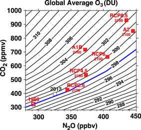
Figure 3. As in figure 3 except for global area-weighted average ozone column (in DU). The dashed square, labeled 2013, is the value that the model would indicate for ozone if the chlorine concentration had been 2 ppbv. The heavy blue line is the 1960 global average column amount of ozone of 298 DU.
Download figure:
Standard image High-resolution imageGSFC2D simulates an increase of around 0.1 × 10¹⁶ molecules/cm2 in global NOy between 1960 and 2100 for the A1B scenario (figure 1), which has been considered in many previous modeling studies. This corresponds to around a 5% increase in global NOy, which is much less than the 25% increase in the N2O boundary condition. This small increase in global NOy for the A1B scenario is consistent with simulations by the three-dimensional CCMs that participated in CCMVal-2. The average change in globally integrated NOy between 1960 and 2100 for the A1B scenario is −2% ± 5% for the 14 CCMs in CCMVal-2. The change in global-average NOy is the net effect of the positive and negative regions integrated over the globe (e.g., Oman et al 2010), and models with a slightly different balance of NOy production and loss will get a slightly different answer. The change is small for all models.
For the other IPCC scenarios there are somewhat larger increases in NOy, but in all cases the percentage increases in global NOy are much smaller than would be obtained for constant CO2. The impact of climate (temperature and circulation) change is seen clearly for scenarios with similar N2O and larger increases in CO2, i.e., compare RCP4.5 and A1B, A2 with RCP8.5.
4. Ozone (O3)
We now consider the change in global column amount of ozone from the suite of GSFC2D simulations. Figure 3 shows the global average O3 as a function of N2O and CO2. As for global-average NOy, the sign of the change in ozone differs between increasing N2O and increasing CO2. Global column amount of ozone decreases with increasing N2O and fixed CO2, but increases with increasing CO2 and fixed N2O. When the increase in CO2 is large and the N2O increase is small there is an increase in total ozone, whereas if there is a large N2O increase and small CO2 change then there can be a decrease in ozone.
It is important to note that changes in O3 shown in figure 3 are due not only to changes in NOx chemistry but also to changes in other ozone loss cycles. In particular, as the stratosphere cools (due to increased CO2) there is a decrease in the ozone loss via each of the loss cycles. In particular, the Ox and NOx cycles are strongly temperature dependent while the ClOx and HOx cycles are significantly less temperature dependent (see e.g. Stolarski et al (2012)). Figure 4 illustrates the dependence of the contributions of the catalytic cycles as a function of the CO2 concentration. The importance of the NOx cycle thus decreases relative to the other cycles as the temperature cools due to CO2 increases.

Figure 4. Fraction of globally-averaged ozone loss due to each catalytic loss cycle as a function of the CO2 boundary condition (BC) in the model simulation. The loss fraction for each cycle has been normalized to its value at 280 ppmv of CO2. The total is indicated by the heavy black line, showing a decrease to about 88% of its 280 ppmv value when the CO2 boundary condition reaches 840 ppmv. The fractions for the Ox and NOx cycles decrease more rapidly than the total because these are the most temperature-sensitive cycles. The fractions for the ClOx and HOx cycle decrease less (small increase for HOx) because these are the least temperature-sensitive cycles.
Download figure:
Standard image High-resolution image
As in figure 1, the open red symbol in figure 3 shows the observed values of N2O and CO2 in 1960, while the values of N2O and CO2 from various scenarios for the year 2100 are indicated by the filled red squares. The simulation using the 1960 concentrations of N2O and CO2 (291 and 316 respectively) yielded a global average ozone column of 298 DU as indicated by the open red box and the heavy blue line. For all of the scenarios the global-average ozone in 2100 is greater than that in 1960. The largest increase (5 DU) occurs for A1B, whereas there is only a very small increase for RCP2.6. This 'super-recovery' of column ozone occurs primarily in the mid and high latitudes with little change in the tropics (e.g., Li et al 2009).
Caution is required interpreting the results shown in figure 3 as they are from a single model and are for steady state calculations. However, these results are consistent with the 1960 to 2100 transient simulations from GSFC2D and other models. First, the 5.1 DU increase in global ozone from 1960 to 2100 in the GSFC2D model transient A1B simulation (Fleming et al 2011) is consistent with the steady-state calculation shown in figure 3. The global ozone difference from 3D CCMs is also of similar magnitude; the multi-model mean increase in ozone for the A1B scenario is 4 ± 2 DU for the 17 CCMs in CCMVal-2 (Eyring et al 2010a, 2010b). Furthermore, sensitivity studies from a small subset of CCMs show a similar dependence of global ozone on N2O and CO2. For example, the changes in ozone for simulations of the different RCPs vary from slight decrease in global ozone for RCP2.6 to a ∼6 DU increase for RCP8.5 (Eyring et al 2007), compared to slight increase to ∼4 DU increase in figure 3. Revell et al (2012b) performed a series of transient simulations with N2O following the different RCP scenarios but CO2 and CH4 following the A1B scenario, and show 2100 global ozone for RCP2.6 (N2O = 344 ppbv) to be 6.7 DU larger than in RCP8.5 (N2O = 435 ppbv). Again, this difference is similar to that in figure 3 (for N2O increasing from 340 to 445 ppbv with CO2 ∼ 700 ppmv). Note that the results for RCP2.6 and RCP8.5 shown in figures 2 and 3 are not directly comparable to the results obtained by other models because our boundary condition for CH4 is constant (1.8 ppmv). Our results are designed to show the model response for the N2O/CO2 relationship without the complicating factor of changes in CH4. We have run simulations for varying levels of CH4 and find that global ozone increases by 3–4 DU per ppm of CH4. The exact amount depends on the amounts of CO2 and N2O. For RCP8.5, the CH4 mixing ratio reaches about 3.5 ppmv by 2100. This results in an extra 6–7 DU of total ozone above the amount shown in figure 3. For RCP2.6, the CH4 mixing ratio in 2100 is reduced to about 1.2 ppmv resulting in a decrease of 2–3 DU in the deduced total ozone from our model simulations.
5. Conclusions
We performed a series of steady-state simulations with the GSFC2D model to examine the potential future control of the ozone layer, focusing on the year 2100 when the concentrations of chlorine and bromine species will have declined due to the continued implementation of the Montreal Protocol. These simulations show that global-average NOy and O3 respond oppositely to increasing N2O and increasing CO2. Global NOy increases and ozone decreases with increasing N2O and fixed CO2, whereas NOy decreases and ozone increases with increasing CO2 and fixed N2O. Thus, the responses of NOy and ozone to increases in N2O are coupled to increases in CO2 and climate change.
These simulations indicate that for all of the GHG scenarios considered in recent IPCC assessments there will only be a small change in global NOy and O3 for conditions in the year 2100 compared to the year 1960. The GSFC2D models shows small increases in global NOy for all IPCC scenarios, with the percentage change significantly smaller than the increase in the N2O mixing ratio imposed at the lower boundary of the model. This occurs because the total amount of NOx available for catalytic ozone loss depends on the amounts of both N2O and CO2 assumed at the lower boundary of the model.
For all scenarios, we also simulate a small increase (∼0–5 DU) in global O3 in 2100 compared to that in 1960 for constant CH4. This increase occurs mainly because of the projected increases in CO2 and despite projected increases in N2O. Taking CH4 variation into account, we obtain a slight decrease (∼2 DU) in global O3 in 2100 for the RCP2.6 scenario because of the projected decrease in CH4 in this scenario.
Although N2O will likely be the most important anthropogenic ODS by the end of the 21st century (Ravishankara et al 2009) and decreases in global ozone are to be expected for an N2O increase at constant CO2, the simulations presented here suggest that increases in N2O will only lead to large reductions in global O3 in the unlikely situation where CO2 concentrations are held constant while N2O concentrations continue to grow rapidly.
Acknowledgments
We thank Charles Jackman and Eric Fleming for making the code of the GSFC2D model available for these calculations.