

Abstract
Microplastic debris floating at the ocean surface can harm marine life. Understanding the severity of this harm requires knowledge of plastic abundance and distributions. Dozens of expeditions measuring microplastics have been carried out since the 1970s, but they have primarily focused on the North Atlantic and North Pacific accumulation zones, with much sparser coverage elsewhere. Here, we use the largest dataset of microplastic measurements assembled to date to assess the confidence we can have in global estimates of microplastic abundance and mass. We use a rigorous statistical framework to standardize a global dataset of plastic marine debris measured using surface-trawling plankton nets and coupled this with three different ocean circulation models to spatially interpolate the observations. Our estimates show that the accumulated number of microplastic particles in 2014 ranges from 15 to 51 trillion particles, weighing between 93 and 236 thousand metric tons, which is only approximately 1% of global plastic waste estimated to enter the ocean in the year 2010. These estimates are larger than previous global estimates, but vary widely because the scarcity of data in most of the world ocean, differences in model formulations, and fundamental knowledge gaps in the sources, transformations and fates of microplastics in the ocean.
Export citation and abstract BibTeX RIS
1. Introduction
Plastic debris has been documented in all marine environments, from coastlines to the open ocean (Barnes et al 2009), from the sea surface to the sea floor (Schlining et al 2013), in deep-sea sediments (Woodall et al 2014) and even in Arctic sea ice (Obbard et al 2014). The best-measured reservoir of plastic marine debris on a global scale is that of buoyant plastics floating at the sea surface. Yet observational data, even in the extensively surveyed Western North Atlantic Ocean (Law et al 2010) and Eastern North Pacific Ocean (e.g. Goldstein et al 2012, Law et al 2014), have not yet determined the full extent of large accumulations of debris associated with the converging surface currents in ocean subtropical gyres. In the Southern hemisphere gyres there are scarcely enough data to confirm the presence of floating plastic debris (Eriksen et al 2013, 2014, Cózar et al 2014), and the vast majority of the sea surface outside the gyres remains unsurveyed, introducing potentially large errors in global estimates of the amount of floating plastic.
Little is known about the transformations of plastics in seawater, including the time scales of degradation and its ultimate sinks. Weakened by UV radiation, chemical degradation, wave mechanics and grazing by marine life, plastics fragment into smaller and smaller pieces; plastic particles smaller than 5 mm in size are commonly referred to as microplastics. It has been suggested that plastic never fully degrades, yet expected increases in plastic concentration in response to increased production and use have not been consistently observed (e.g. Thompson et al 2004, Law et al 2010), and global budgeting exercises find less material on the ocean surface than expected (Cózar et al 2014, Eriksen et al 2014). To properly evaluate the risk of plastic contamination to marine organisms, understanding the amount, form and distribution of plastic in the marine environment, and how these evolve in time, is necessary. In this study, we focus on assessing the amount and distribution of 'small' (nominally <200 mm) plastic debris on the ocean surface, as these are by far the most sampled data set and also have demonstrated biological impact (Rochman et al 2015), although larger items can also impact biota.
At the sea surface, microplastic marine debris is typically measured by surface-towing plankton nets with mesh ranging from 0.1 to 0.5 mm, which capture particles limited to the size of the net aperture. Net tow sampling efforts typically capture plastic particles smaller than 10 mm in size (Morét-Ferguson et al 2010), while less numerous larger items are observed by visual surveys with ships or aircraft. The vast majority of observations since the 1970s have been made using plankton nets, with broadly similar sampling methodologies but variable reporting units (particle count per area or volume, or mass per area or volume). In contrast, visual surveys of macroplastic debris are conducted using a wide range of survey protocols ranging from (non-quantitative) opportunistic sightings to rigorous distance sampling methods (e.g. Williams et al 2011) for which it is difficult to satisfy all underlying methodological assumptions (Buckland et al 2001). In addition to the difficulty in reconciling different visual survey techniques (although useful reference standardized approaches based on distance sampling have been proposed, e.g. Ryan 2013), large debris is less numerically abundant than microplastics and its drift behavior and accumulation patterns are likely quite different because of its size, buoyancy and windage. Even though large debris accounts for a substantial mass of ocean plastics, for the reasons described above, we consider only data from plankton net trawls, which primarily collect microplastics in this analysis.
With the recent addition of relatively large and more geographically widespread datasets, and oceanographic numerical models that predict debris accumulation at the sea surface from surface current patterns, the first global estimates of the reservoir of floating plastic debris have recently been reported (Cózar et al 2014, Eriksen et al 2014). Using plankton net data (1127 trawls) spatially averaged in accumulation and non-accumulation zones defined from a statistical oceanographic model (Maximenko et al 2012), Cózar et al (2014) estimated between 7000 and 35 000 tons of floating plastic (0.20–100 mm in size) in the Atlantic, Pacific and Indian Oceans combined. Using a nearly independent plankton net dataset (680 trawls), Eriksen et al (2014) computed a global estimate of floating plastic (0.33–200 mm in size; 66 140 metric tons) using a different oceanographic model (Lebreton et al 2012) whose output was scaled by the globally measured plastic concentration. Given the methodological differences between these studies, it is encouraging that the resulting estimates are so close.
Here we estimate the global standing stock of small floating plastic debris with the most comprehensive dataset, ocean models and ocean plastic input estimates available. We compiled all available plastic data collected with surface-trawling plankton nets (more than 11 000 observations, including those in Cózar et al 2014 and Eriksen et al 2014), resolved sampling biases and other variations using a statistical model, and then used the standardized dataset to scale the outputs of three ocean circulation models. By comparing the three scaled model solutions, we assessed where debris patterns are well predicted and identified regions where discrepancies between solutions must be resolved through improved process description in models, additional oceanographic data collection and/or increased understanding of sources, composition, and lifecycle of plastic debris.
2. Methods
2.1. Plankton surface-trawl dataset
Plankton nets can capture any debris larger than the net mesh and smaller than the net mouth, but net dimensions vary between studies and maximum particle size is often not reported. Since most particles collected in plankton nets are millimeters in size or smaller, from here forward we use the term 'microplastics' not in its strict definition (as particles <5 mm in size), but instead to conveniently refer to all plastic debris collected in surface-trawling plankton nets.
There are two relevant measures for net-collected plastic debris: particle count and mass. Both have their merits. Samples are easier to count than to weigh, especially while underway at sea, and the number of particles may be more relevant for an exposure assessment. On the other hand, as a conservative variable, mass can more easily be related to source estimates, and will eventually be needed to close the mass balance of ocean plastics. Because of these considerations, we report both measures.
Plastic data collected using surface-trawling plankton nets were identified by literature search and data were assembled either directly from the publication or by contacting the corresponding author (table S1). Additional unpublished data were provided by contributing authors. In total 27 floating debris studies were identified, with 11 854 surface trawls carried out between 1971 and 2013, spanning all major ocean basins except the Arctic. Given the long time span over which samples were collected, we addressed sampling year as a potential bias when we standardized the data (see section 2.2). Net mesh ranged from 0.15 to 3.0 mm in size, although more than 90% of observations were collected using a manta net or neuston net with 0.333 or 0.335 mm mesh. Most studies did not report the maximum size of plastic debris collected. All data reported in units of #m−3 were converted to #m−2 by multiplying by the submerged height of the net, and then cast into units of #km−2. Nearly all studies reported plastic abundance in count units, and two-thirds reported data in mass units. However, the three largest datasets (comprising 82% of total observations) only reported counts. Conversions to mass for datasets in which only count was reported were made using factors derived from empirical data collected in similar geographic regions, during similar time periods and/or using similar sampling methods (table S1).
Microplastic abundance at the sea surface has been shown to vary with wind speed due to vertical mixing (Kukulka et al 2012, Reisser et al 2015), yet most studies did not report wind data. To evaluate the relationship between wind speed and plastic abundance as a source of variability in the data set, we used daily-averaged wind speed from the ECMWF ERA-Interim global atmospheric reanalysis (Dee et al 2011) interpolated to each surface trawl date and location. ERA-Interim output is available beginning 1 January 1979; thus, 222 surface trawls collected prior to 1979 were omitted from our analysis.
2.2. Data standardization using statistical modeling
Microplastics sampled were collected in a wide range of conditions over a multi-decadal period. Before scaling ocean circulation model outputs with these data, we first removed variability associated with factors that could affect either the concentration of plastic in the ocean or the representativeness of the samples, such as sampling year, wind speed, distance of the tow, and others. We used a generalized additive model (GAM; Wood 2006), implemented in the R statistical language (R Core Team 2013), to estimate the relationships between these variables and the observed plastic concentration (in counts), and then used those relationships to adjust the observations to represent standardized conditions.
We first created a base model using a spherical smooth term (two-dimensional spline) to represent location on the globe, assuming that repeated samples in the same location should share an underlying average value. We then explored the effects of sampling year, wind speed, trawl length, and study ID on measured plastic concentrations. To account for changes in time we explored incorporating either a smooth term or first and second order polynomials with year since 1950, approximately the beginning of commercial plastic production, to allow for nonlinearity in the relationship. We did the same to evaluate the sampling bias associated with variable wind speed. We used the model residuals to diagnose any locations of poor fit in the model, in particular those resulting from discontinuities between sampling regions caused by land. Where we found these issues, we allowed a transition in the spatial surface by incorporating a nonlinear function of the distance from the discontinuity as a predictor variable.
We defined the set of potential GAMs a priori and used the Akaike information criterion (AIC; Burnham and Anderson 2002) to determine the best model, balancing parsimony and fit across the full set of possible models. We chose a Tweedie distribution with a parameter of 1.6 to allow for over-dispersion in the data. The best performing GAM was used to predict the plastic concentrations that would have been observed for each sample had it been taken under no-wind conditions in the year 2014 (hereafter the 'standardized dataset'). We also estimated the standard error in our predictions based on the variance-covariance structure among the fitted parameters, using the tools provided in the mgcv package (Wood 2006). These standard errors were used to estimate the 95% confidence intervals on the standardized plastic concentrations. Where calculations required values in mass, as opposed to counts, we used the ratio of mass to count from the observational data (as originally reported or using the conversion factors discussed above) to convert standardized counts to standardized masses.
2.3. Ocean circulation models
The non-uniformly distributed, standardized plastic concentrations must be spatially interpolated in order to produce a global map of microplastic distribution. This is particularly important in regions of low coverage, such as in the Southern Hemisphere. While in principle this could be done with simple interpolation methods such as kriging, more realistic results can be obtained by synthesizing observations with ocean circulation model predictions. In order to assess the dependence of the resulting global microplastic distribution on the choice of ocean circulation model, we used three largely independent models. As in Maximenko et al (2012), Lebreton et al (2012) and van Sebille et al (2012), we released virtual microplastic in ocean circulation models to obtain maps of likely distribution of microplastics from transport by ocean surface currents. Each model-predicted distribution provides one regression parameter per basin. The results of this regression exercise depend on the assumptions made in each ocean circulation model, such as how surface currents are derived, how plastic is released into the ocean, and whether and how microplastics are removed from the surface.
The Maximenko model (Maximenko et al 2012) uses a transition matrix approach, based on the probability of particle travel between ½° bins calculated from trajectories of a historical global set of satellite-tracked drifting buoys (http://aoml.noaa.gov/phod/dac/index.php). Microplastics, represented as a virtual tracer, are advected through the ocean by iterating the transition matrix for 10 years. As a source function, this model used a uniform distribution of microplastics over the global ocean. They showed that in 2 to 3 years a high concentration of microplastics builds up in the five subtropical gyres, where it creates spatial patterns not sensitive to the initial condition, and with the potential to persist for hundreds of years before washing ashore.
The Lebreton model (Lebreton et al 2012) uses ocean velocity fields from the 1/12° global HYCOM circulation model. Virtual microplastics are sourced on major river mouths as a function of urban development (impervious surface area) within individual watershed, on coastlines as a function of coastal population, and on major shipping routes as a function of shipping traffic. Here, we use the coastal population scenario only, for consistency with the van Sebille model (below). Microplastics are continuously released in increasing amounts based on global plastic production data (Plastinum 2009) and are advected by the ocean surface velocity field for thirty years.
Finally, the van Sebille model (van Sebille et al 2012, van Sebille 2014) also advects microplastics in ocean currents captured in a transition matrix built from the trajectories of drifting buoys, as in the Maximenko model. Here, the source function is assumed to be proportional to the human population within 200 km of the coast, scaled by the amount of plastic waste available to enter the ocean by country in 2010 (Jambeck et al 2015, what they term 'mismanaged waste'). Microplastics are continuously released at each coastal point over 50 years (1964–2014), increasing in time based upon global plastic production data (Plastics Europe 2013).
All three ocean circulation models treat microplastic sinks differently. While the Lebreton and van Sebille models have no sinks at all (i.e., all released microplastic stays in the ocean indefinitely), microplastics in the Maximenko model can 'wash ashore' when they enter grid cells with a model shoreline. None of the models incorporate loss of surface microplastics from the open ocean by sinking or ingestion because there is insufficient data on these open-ocean loss rates. Furthermore, the models do not incorporate fragmentation and therefore treat particle count concentrations similar to mass concentrations.
The global microplastic distribution fields for the year 2014 from each of the three models were interpolated to a common 1° × 1° resolution and divided into six separate basins (the North and South Pacific, the North and South Atlantic, the Indian, and the Mediterranean). For each basin and each model, the model prediction value was compared to the standardized plastic counts and mass at each of more than 11 000 locations. This yielded, for each basin and model, a regression coefficient used to scale the (unitless) model microplastics distribution to a solution of global microplastics abundance in units of particles km−2 and g km−2.
3. Results
The best-fitting GAM for the data standardization includes a two-dimensional spatial spline, a year term, first and second order terms for wind speed, and a discontinuity at the Americas between the Caribbean and Pacific basins (table 1). The region between the Caribbean and Pacific basins was the only portion of the sampling space where the number of samples and their proximity required incorporation of a spatial discontinuity, based on examination of the residuals from the model. The distance of the net tow was not a significant source of variability in the samples. Based on deviance, the final model explains 71.6% of the variation in observed plastic counts. The coefficient for sampling year is positive and significant, indicating increasing plastic concentrations over time. The wind terms indicate a negative but asymptotic relationship between plastic concentrations and wind speed (table 1). The coefficient for the discontinuity at the Americas is not significant; however, based on AIC scores it significantly improved the model fit to the data and is therefore included.
Table 1. Adequacy of the candidate standardization models and coefficients of the best fitting model.
| A. Model fit | B. Best fit model coefficients | ||||
|---|---|---|---|---|---|
| Model | AIC | Coefficient | Estimate | Std err | p value |
| SAyWWsqBd2 | 159533.3 | Intercept | 7.3 | 3.4 | 0.033 |
| SAyWWsqBd | 159537.7 | Year (since 1950) | 0.016 | 0.005 | 0.0012 |
| SAyWWsq | 159538.2 | Wind Speed | −0.34 | 0.045 | 1.40 × 10⁻¹³ |
| SAyWBd | 159541.9 | Wind speed squared | 0.011 | 0.0044 | 0.015 |
| SAyWBd2 | 159541.9 | Atlantic–Pacific boundary squared | 3.7 | 8.4 | 0.67 |
| SAyW | 159542.4 | ||||
| SWWsq | 159592.8 | ||||
| SW | 159598.4 | ||||
| SWsq | 159727.7 | ||||
| S | 160546.3 | ||||
| 0 | 177503.4 | ||||
Note: model codes in panel A are: 0—intercept only, S—spherical smooth, W—wind speed, Wsq—wind speed squared, Bd—Caribbean–Pacific discontinuity, Bd2—Caribbean–Pacific discontinuity squared, Ay—Sampling Year (since 1950). Lower AIC indicates an improved model, with a difference of 2 units suggesting statistically significant improvements.
In the standardized data, surface microplastic counts and mass varies by several orders of magnitude (figure 1). The highest concentrations are in the centers of the subtropical gyres, mainly in the North Atlantic and North Pacific, where plastic particles accumulate due to convergence of Ekman transports (Kubota 1994, van Sebille 2015). Concentrations are much lower in the tropics, poleward of 45°S and 45°N, and in the remote coastline off Western Australia (Reisser et al 2013). Microplastic counts and mass have similar patterns, although counts yield a 'smoother' field, especially in the Southern Hemisphere.

Figure 1. The location and standardized (a) microplastic count and (b) microplastic mass of all surface trawl data used in this analysis, on a log10 scale. Standardization is done with respect to year of study, geographic location, and wind speed. The spatial term includes a discontinuity at the Americas to allow for differences between the Caribbean Sea and tropical Pacific Ocean. Compare to figure S1 for the raw, un-standardized data.
Download figure:
Standard image High-resolution imageThe three ocean circulation models scaled with the standardized data (hereafter 'model solutions') reasonably demonstrate the large variability in microplastic concentrations, and accurately capture the highest values (> ∼105 particles km−2, figure 2(a)). However, the observed microplastic concentrations are much higher than the model solutions for concentrations below 104 particles km−2. This bias could result from the detection limit in surface trawls; the lowest observable microplastic concentration above zero is 1 piece per trawl, which is equivalent to 540 particles km−2 for a typical surface trawl of 1 nautical mile (van Franeker and Law 2015). The standardization typically increases these values (figure S2), enhancing the bias. In contrast, the models have no such limit and can reach much lower non-zero values. Beyond this obvious discrepancy between solutions and observations, there is a mismatch in the North Atlantic, where all models predict the highest concentrations around 60°W (figure 3), whereas the highest observed concentrations are farther East (figure 1).

Figure 2. (a) Comparison between the three ocean models and the standardized observations (top row), and (b) inter-comparison between the three ocean models (bottom row), at each surface trawl location. The points are color coded according to basin, and the black lines are the one-to-one lines. The correlations reported in the top row give an estimate of agreement between the models and observations. All models reach much lower microplastic counts than the observations, likely because of detection limits of surface trawls (see text). The van Sebille model gives slightly higher values than the other two models, particularly for regions where microplastic counts are low.
Download figure:
Standard image High-resolution image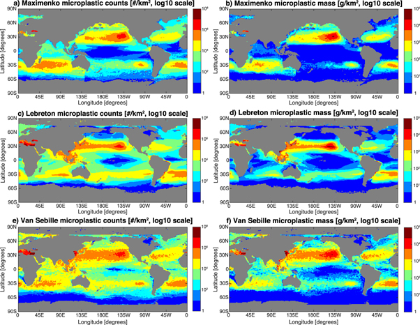
Figure 3. Maps of the solutions of microplastic count (left column) and mass (right column) distribution for the three different models. Because fits are done on a per-basin level, there are a few discontinuities visible (e.g. South of Tasmania in the Maximenko solution, panel (a).
Download figure:
Standard image High-resolution imageThe van Sebille solution is skewed high compared to the other models, especially at very low concentrations (figure 2(b)). This appears to be related to the source function of the van Sebille model, where microplastics are continuously released on an exponential growth curve, resulting in high concentrations even in regions of strong divergence. The skewedness disappears when the van Sebille model is rerun with a one-time release of microplastics (figure S3), although the Lebreton model also has an increasing source function over time.
The microplastic count and mass patterns broadly agree across model solutions (figure 3), with all three showing high values in the subtropics and low values in the tropics and high latitudes. There are regional differences in high concentration areas such as the South Pacific, where the Maximenko solution has lower concentrations, and the North Atlantic, where the Lebreton solution has lower concentrations. In the Indian Ocean the Lebreton solution has lower concentrations and also has peak concentrations in the Eastern rather than Western basin like the other two models.
The largest differences between the three solutions occur in low concentration regions, visualized by calculating the ratio between highest and lowest solutions (in counts) at each point (figure 4). Solutions differ by more than a factor of 100 in the tropics and at high latitudes, whereas solutions in the centers of the accumulation zones differ by less than a factor of 10. The solutions also differ strongly in the Mediterranean, where the Lebreton and van Sebille models project very high microplastic concentrations in the Eastern basin, in contrast to the coarse-resolution (½°) Maximenko model, which was not designed for such small basins.

Figure 4. Map showing the level of agreement between the three different models, in terms of microplastic counts. Pink shading denotes areas where the lowest and highest estimates differ by less than a factor of 10; red shading denotes areas where the lowest and highest estimates differ by between a factor of 10 and 100; and dark red shading denotes areas where the lowest and highest estimates differ by more than a factor of 100. The three models agree reasonably well within the centers of the gyres, but strongly differ in the tropics, the high latitudes, and the Eastern Mediterranean.
Download figure:
Standard image High-resolution imageOne reason for the discrepancies between model solutions could be the source function, which is continuous in time and non-uniformly distributed in space in the van Sebille and Lebreton models, compared to the single initial release of evenly distributed microplastic in the Maximenko model. This might also explain the much lower concentrations near Asian coastlines and in the Mediterranean in the Maximenko solution. Another difference is the intra-annual variation in the statistics of ocean currents that is not accounted for in the Maximenko model, which could distort diffusion of particles from the high concentration gyres.
The three different model solutions can be aggregated by basin to yield total microplastic counts and mass (figure 5, tables 2 and 3), with black error bars representing the 95% confidence interval (see section 2.2) and gray error bars representing the 95% confidence interval of both the standardization procedure and the linear regression. For most basins the error bars are as large as, or larger than, the differences between the three solutions, with the North Atlantic and Mediterranean as exceptions.

Figure 5. Bar plot of (a) the total amount of microplastic particles in each of the basins and (b) the total mass of microplastics in each of the basins in units of thousand metric tons, for the three different model solutions for 2014. Error bars indicate 95% confidence intervals, with the black bars the error due to the standardization, and the gray bars the error due to the standardization and the linear regression. The purple dots in (b) are the basin-summed estimates of the amount of plastic waste available to enter the ocean in 2010 (Jambeck et al 2015), in units of hundred thousand metric tons (note scale difference from total microplastic mass). All models predict the largest microplastic mass in the North Pacific Ocean. While there are a large number of particles in the Mediterranean basin (in the Lebreton and van Sebille model), they have a very small average mass (table S1) and therefore do not account for much of the total mass. The largest differences between the models are in the Mediterranean Sea, and to a lesser extent in the North Pacific and Atlantic basins. The models agree quite well on the amount of microplastic particles in the Indian and South Pacific basins.
Download figure:
Standard image High-resolution imageTable 2. Overview of the modeled microplastic count solutions per basin, in 1012 particles. For each of the three models, the best estimates as well as the 95% confidence intervals related to both the standardization (Stand C.I.) and regression (Regr C.I.) are given.
| Count | Maximenko model | Lebreton model | van Sebille model | ||||||
|---|---|---|---|---|---|---|---|---|---|
| (1012 particles) | Best Est | Stand C.I. | Regr C.I. | Best Est | Stand C.I. | Regr C.I. | Best Est | Stand C.I. | Regr C.I. |
| N Pac | 7.3 | 1.2 | 0.1 | 9.4 | 1.7 | 0.5 | 15.9 | 2.7 | 0.4 |
| S Pac | 0.3 | 0.1 | 0.0 | 0.7 | 0.4 | 0.1 | 0.8 | 0.4 | 0.0 |
| N Atl | 0.4 | 0.1 | 0.0 | 0.3 | 0.1 | 0.0 | 1.3 | 0.3 | 0.1 |
| S Atl | 1.0 | 0.3 | 0.2 | 2.6 | 0.9 | 0.3 | 2.0 | 0.7 | 0.1 |
| Ind | 2.8 | 1.7 | 0.3 | 2.0 | 1.3 | 0.5 | 3.0 | 1.9 | 0.6 |
| Med | 3.2 | 0.5 | 0.3 | 16.1 | 2.5 | 1.5 | 28.2 | 4.4 | 4.8 |
| Total | 14.9 | 2.1 | 0.5 | 31.2 | 3.4 | 1.7 | 51.2 | 5.6 | 4.9 |
Table 3. Overview of the modeled microplastic mass solutions per basin, in thousand metric tons. For each of the three models, the best estimates as well as the 95% confidence intervals related to both the standardization (Stand C.I.) and regression (Regr C.I.) are given.
| Mass | Maximenko model | Lebreton model | van Sebille model | ||||||
|---|---|---|---|---|---|---|---|---|---|
| (Thousand metric tons) | Best Est | Stand C.I. | Regr C.I. | Best Est | Stand C.I. | Regr C.I. | Best Est | Stand C.I. | Regr C.I. |
| N Pac | 62.8 | 10.9 | 11.9 | 108.2 | 20.7 | 22.4 | 155.2 | 28.0 | 28.2 |
| S Pac | 1.0 | 0.5 | 0.1 | 3.7 | 1.8 | 0.4 | 3.7 | 1.8 | 0.3 |
| N Atl | 5.1 | 1.1 | 0.7 | 3.6 | 0.8 | 0.7 | 17.7 | 3.8 | 1.6 |
| S Atl | 6.2 | 2.1 | 2.5 | 15.5 | 5.4 | 5.8 | 14.2 | 5.0 | 3.6 |
| Ind | 13.3 | 8.3 | 6.6 | 5.5 | 3.5 | 7.5 | 15.0 | 9.6 | 8.4 |
| Med | 4.8 | 0.7 | 1.6 | 15.0 | 2.3 | 5.9 | 30.3 | 4.9 | 11.9 |
| Total | 93.3 | 13.9 | 14.0 | 151.5 | 21.9 | 25.0 | 236.0 | 30.7 | 32.0 |
The highest microplastic counts are in the Mediterranean (two solutions) and the North Pacific, while the largest microplastic mass is in the North Pacific in all three solutions. The total mass in the Mediterranean is much smaller because of the very small average particle mass and much smaller basin size. Surprisingly, the North Atlantic has low microplastic counts in all three solutions, and the lowest count and mass of any basin in the Lebreton model. This likely results from the relatively poor correlations between solutions and observations for this basin (figure 2), where the models do not achieve high enough concentrations in the center of the gyre.
The patterns of the basin-summed microplastic abundances in the three models are consistent with the basin-summed estimated total plastic waste available to enter the ocean in 2010 from Jambeck et al (2015), which was used as a source function in the van Sebille model, but not in the other two models. With the exception of the Indian Ocean, the basin-summed microplastic mass is on the order of 1% of the estimated amount of plastic waste available to enter each basin in 2010. The smaller fraction in the Indian Ocean may be due to that basin being the most 'leaky', with a microplastic residence time of only a few years (van Sebille et al 2012).
The three solutions can be used to investigate the global abundance and distribution of microplastics (tables 2 and 3). The van Sebille model yields the highest total microplastic concentration (51.2 × 10¹² particles) and mass (236 thousand metric tons), followed by the Lebreton model (31.2 × 10¹² particles, 152 thousand metric tons) and the Maximenko model (14.9 × 10¹² particles, 93.3 thousand metric tons). The Lebreton and van Sebille estimates are not different at the 95% confidence interval (bars in figure 6), while the Maximenko estimate is significantly lower, likely because of the single particle release combined with particle removal at coastlines. Even the lowest of the model solutions is substantially larger than the global microplastics estimates by Cózar et al (2014) (7 thousand to 35 thousand tons) and Eriksen et al (2014) (5.25 × 10¹² particles, 66.1 thousand metric tons for particle sizes up to 200 mm).

Figure 6. Cumulative frequencies of microplastic concentrations, for the three different model solutions. The shaded areas represent the 95% confidence interval due to the standardization (darkest hues and black lines) and due to both the standardization and the regression (lightest hues and gray lines). For example, in the Lebreton solution, 50% of the microplastic is in regions of the ocean where microplastic concentrations are lower than 2 × 10⁶ particles km−2, whereas in the Maximenko solution 50% of the particles are in regions where microplastic concentrations are lower than 4 × 10⁵ particles km−2. Between 30% (Lebreton) and 70% (Maximenko) of particles reside in regions of low concentration (<106 particles km−2).
Download figure:
Standard image High-resolution image
The highest concentration of microplastics in any solution is 108 particles km−2 in subtropical gyres, yet median concentrations range from 4 × 10⁵ particles km−2 (Maximenko solution) to 2 × 10⁶ particles km−2 (van Sebille solution) (figure 6). This implies that 50% of microplastics are in relatively low concentration regions. For example, if accumulation zones are defined by microplastic concentrations greater than 106 particles km−2, then between 30% (Lebreton solution) and 70% (Maximenko solution) of the microplastic resides outside these zones.
The solutions are dependent in part on the distribution of observational data. In all basins surface trawls tend to be clustered in relatively small regions, mostly in the accumulation zones themselves (figure 1); thus, the regression between observations and model fields is biased towards agreement in these high concentration areas. To mitigate this effect we also computed solutions by fitting to observations inversely weighted by the number of observations in each grid cell, thereby putting more emphasis on observations in less-sampled areas. The resulting total microplastic counts and mass (figure S4) show the same general pattern, but are slightly lower than the unweighted version and have slightly smaller error bars (table S2). The exception is the Maximenko solution for mass, which increases slightly.
4. Discussion and conclusions
A major objective of this analysis is to inform the abundance and distribution of plastic debris in the ocean in order to ultimately assess marine animals' exposure to and impact from interaction with debris. Ours is the third study to estimate the amount and distribution of small floating plastic particles in the global ocean, using the largest dataset to date and three different ocean circulation models. While the previous two studies found coarse agreement in the global mass of plastics collected using surface-trawling plankton nets (7–35 thousand tons by Cózar et al 2014; 66 thousand metric tons by Eriksen et al 2014), our model solutions not only exceed these but also vary substantially from 93 to 236 thousand metric tons.
Despite the wide discrepancy in these standing stock estimates, all analyses find the highest concentrations of net-collected plastics in the subtropical gyres, with the largest mass reservoir in the North Pacific Ocean, presumably because of its vast area and also the large inputs of plastic waste from coastlines of Asia and the United States (Jambeck et al 2015).
To a considerable extent, our mass estimates may be larger than previously published estimates because of the data standardization used. Adjusting each observation forward in time to a common sampling year of 2014 and to no-wind sampling conditions increased the observed plastic concentrations in nearly all samples (figure S2). Previous studies have taken vertical wind-mixing of buoyant plastic debris into account by employing a simple one-dimensional model (Kukulka et al 2012) whose dynamics capture only a fraction of deep mixing observed (Brunner et al 2015). Certainly the variation in data collection (e.g., net mesh size); sample analysis (e.g., visual versus microscope identification); count-to-mass conversions (which are strongly dependent on particle size); and model design (e.g., source functions and removal processes) also contribute to the discrepancies.
The variation in model solutions in our study emphasizes that most of the ocean surface is undersampled for microplastics. Uncertainties in the Southern Hemisphere basins illustrate the lack of data even in high concentration subtropical gyres. The least sampled regions are areas of low plastic concentrations, where models predict between 30% and 70% of particles may reside (figure 6). Perhaps the starkest illustration is in the Mediterranean Sea, where models predict between 21% and 54% of global microplastic particles, equivalent to between 5% and 10% of global mass (because of small average particle size), are located. Our dataset has only 105 surface trawls concentrated in a very small region of the Western basin, whereas models predict the highest concentrations in the Eastern basin. One might expect to find very large plastic concentrations given the predicted large inputs of land-based plastic waste (Jambeck et al 2015) and the very long residence time of surface waters due to lack of exchange with the North Atlantic. Indeed, recent field data not included in this study confirmed very high mean surface concentrations in the Southern Adriatic Sea from 29 surface trawls (1.05 million particles km−2; 442 g km−2; (Suaria et al 2015)), yet more data, especially in the Eastern basin, is strongly needed.
Any global estimate of total accumulated floating microplastic debris is only on order of 1% or less of the amount of plastic waste available to enter the ocean annually from land-based sources. While these source estimates from Jambeck et al (2015) have relatively large uncertainties themselves (for example because they omit the tonnage of plastic locally burned, buried and recovered by self-employed wastepickers), it is hard to see their source and our floating stock estimates converge. While some of the 'missing' mass would be in plastic items larger than 200 mm (e.g. Eriksen et al 2014), and hence not included in our study, this is unlikely to account for the two orders of magnitude difference.
Importantly, however, there is no reason that standing stock estimates should equal an annual input estimate, especially since the input is of all plastic materials, not just those that float. Seafloor deposits of dense plastics, coastal deposits, and debris larger than typically captured in plankton nets are undoubtedly important reservoirs of plastic debris. In addition, standing stock reflects inputs and removal over time. The input rate is a function of not only the amount of plastic entering the ocean, but also of the rate at which these presumably large items fragment into the microplastics that surface trawls mostly collect. Removal processes are hypothesized (Law et al 2010), but their rates are essentially unknown. Multi-decadal time series of industrial resin pellets in the North Atlantic subtropical gyre and in North Sea seabirds indicate that removal can be quite rapid (van Franeker and Law 2015). Microplastics might fragment to as-yet undetectable sizes, sink due to buoyancy loss (Ye and Andrady 1991), be deposited on shorelines (McDermid and McMullen 2004), or be ingested and subsequently reduced in size (e.g., due to digestive grinding) and/or transported to land or the seafloor upon egestion. Biota represent the only other reservoir for which microplastic mass estimates exist. Myctophid fishes in the North Pacific gyre were estimated to hold 12–24 thousand metric tons of microplastic (Davison and Asch 2011), and the growing knowledge on ingestion of plastics by fishes (Kühn et al 2015) could imply a reservoir comparable in size to the sea surface.
The order-of-magnitude discrepancies in these global-scale budgeting exercises reveal a fundamental gap in understanding akin to the 'missing' anthropogenic carbon dioxide in the carbon budgeting exercise of the early 2000s (e.g. Stephens et al 2007). Until these discrepancies are resolved at even a coarse scale, we cannot quantify the full suite of impacts of plastic debris on the marine ecosystem.
Acknowledgments
This work was conducted within the Marine Debris Working Group at the National Center for Ecological Analysis and Synthesis, University of California, Santa Barbara, with support from Ocean Conservancy. We particularly thank George Leonard and Nick Mallos for their support, and Steven D Gaines for thoughtful insights. We thank H Carson, A Cózar, M Doyle, C Fossi, G Lattin, C Panti, R Yamashita, and A Zellers for kind assistance in compiling plankton net data. EvS was supported by the Australian Research Council (DE130101336). BDH and CW were supported by CSIRO's Oceans and Atmosphere Flagship. JAF was supported by IMARES internal funds. NM was partly supported by NASA through grants NNX08AR49G and NNX13AK35G. KLL was supported by the National Science Foundation (OCE-1260403) and Sea Education Association. We thank two anonymous reviewers for their helpful comments. This is IPRC/SOEST Publication 1160/9532.