

Abstract
Leading-edge tubercles on a humpback whale flipper are known to enhance its hydrodynamic performance at post-stall angles of attack (Miklosovic et al 2004 Phys. Fluids 16 39–42). We investigate vortical structures above a three-dimensional wing with tubercles using surface-oil-flow visualization and particle image velocimetry measurement. Two wing models with and without tubercles, previously studied by Miklosovic et al (2004 Phys. Fluids 16 39–42), are considered at the Reynolds number of 180 000 based on the free-stream velocity and mean chord length. At this Reynolds number, tubercles delay the stall angle by 7° and increase the maximum lift coefficient by about 22%. At a low angle of attack, flow separation first occurs near the tip region for both wing models. While flow separation rapidly progresses inboard (toward the wing root) for the model without tubercles with increasing angle of attack, tubercles produce two types of vortical motions and block the inboard progression of flow separation, resulting in delayed stall from α = 8° to 15°. One of these two vortical structures is pairs of counter-rotating streamwise vortices evolving from hemi-spherical separation bubbles near the leading-edge troughs at pre-, near-, and post-stall angles of attack, and the other is asymmetric pairs of streamwise vortices evolving from separated flow regions after the mid-chord region at near-stall angle of attack. At a post-stall angle of attack (α = 16°), strong clockwise and counter-clockwise streamwise vortices are generated from foci at the root and tip near the trailing edge, respectively, and delay flow separation in the mid-span, resulting in a higher lift coefficient than that without tubercles.
Export citation and abstract BibTeX RIS
1. Introduction
Living creatures have long evolved through natural selection to cope with the surrounding environment. In particular, aquatic animals have changed their morphology to move efficiently in water (Fish and Lauder 2006). For example, tubercles on the pectoral flipper of humpback whale enhance the hydrodynamic performance at high angles of attack (Miklosovic et al 2004, 2007); carapace of some species of the boxfish has low drag coefficients and provides self-correcting trimming forces to swim in smoother trajectories (Bartol et al 2003, 2005); scales of a shortfin mako are bristled by reversed flow, preventing flow separation (Lang et al 2014); grooves of scallops increase the lift-to-drag ratio at moderate and high angles of attack (Choi et al 2012); longitudinal ridges of leatherback turtles improve the hydrodynamic performance depending on swimming modes (Bang et al 2016). Especially, the humpback whale has been known as one of the most acrobatic whales in spite of its huge size, and it has been suggested that this agility results from the use of large pectoral flippers which have rounded tubercles along the leading-edge (Jurasz and Jurasz 1979, Fish and Battle 1995). Previous field studies reported that humpback whales exhibit unique feeding behaviours that require tight turnings (Jurasz and Jurasz 1979, Hain et al 1982). Because the path radius is inversely proportional to the lift force, increasing the lift force is important to catch prey with unique feeding behaviours (Weihs 1981, Fish and Battle 1995). Therefore, many researchers have investigated the relationship between the leading-edge tubercles and lift force.
Previous studies on the effects of leading-edge tubercles on the hydrodynamic (or aerodynamic) performance may be categorized into two types depending on the wing (or airfoil) models used, namely two-dimensional (2D) airfoil versus three-dimensional (3D) wing. Studies on 2D airfoils, which were conducted at Re = 50 000–450 000, showed that hydrodynamic performances of 2D airfoils with leading-edge tubercles are better than those without tubercles only in the post-stall region but worse before stall (Johari et al 2007, Miklosovic et al 2007, Hansen et al 2011, Zhang et al 2013, 2014, Cai et al 2015, Custodio et al 2015, New et al 2015). Studies using 3D wing models, however, showed various results depending on the wing planform geometry and Reynolds number. In the case of an idealized humpback whale flipper model which imitated a real humpback whale pectoral flipper and had a back-swept planform geometry, leading-edge tubercles delayed the stall, increased the maximum lift coefficient, and increased the lift and decreased the drag in the post-stall region at Re = 505 000–631 000 (Miklosovic et al 2004, 2007). Stanway (2008), who conducted experiments using a slightly modified humpback whale flipper model with a lower aspect ratio at Re = 44 648–119 060, reported that leading-edge tubercles delay the stall for all Reynolds numbers considered, but increase the maximum lift coefficient only at the highest Reynolds number of Re = 119 060. Bolzon et al (2017a) considered a back-swept wing model with a sweep angle of 35° and a taper ratio of 0.4 at Re = 225 000. They reported that tubercles on the leading-edge little change the stall phenomenon, but decrease the lift for all angles of attack (0°–20°) and the drag at low angles of attack (0°–8°). In addition, they suggested based on velocity measurements in the wake that spanwise locations corresponding to the troughs have local maximum profile drag and minimum induced drag, but those corresponding to the peaks have the opposite result (see also Bolzon et al 2016). Bolzon et al (2017b) also considered an untapered back-swept wing model with the same sweep angle, and showed that the lift and drag are little changed by single tubercle located at the wing tip. Wei et al (2018a) investigated two different back-swept wing models with a sweep angle of 30° and a taper ratio of 0.33 at Re = 220 000. In one model tubercles were aligned with the free-stream direction, but in the other they were normal to the leading-edge. They showed that the tubercles delay the stall but decrease the lift before the stall for both models, but the maximum lift coefficient increases only for the latter model. On the other hand, for the first model, the lift increases for all angles of attack at a lower Reynolds number of Re = 55 000 (Wei et al 2018b). Researches have been also conducted for unswept wings. Weber et al (2010) experimentally investigated the effects of leading-edge tubercles on the hydrodynamic performance of unswept rudders with low aspect ratio of 1.6 and taper ratio of 0.67 at Re = 200 000–880 000. They suggested that there exists a critical Reynolds number of Re = 800 000 above which the effects of leading-edge tubercles disappear. Guerreiro and Sousa (2012) measured forces on unswept finite wing models with low aspect ratios of 1 and 1.5 at Re = 70 000 and 140 000. They showed that leading-edge tubercles increase the lift in the post-stall region at Re = 140 000 when tubercle amplitude and wavelength are properly selected, otherwise the lift is unchanged or decreases for all angles of attack considered. On the other hand, tubercles have favourable effects even at low angles of attack for Re = 70 000. Yoon et al (2011) conducted RANS simulations for an unswept finite wing model with a low aspect ratio of 1.5 at Re = 1000 000. They investigated the effect of Rw (ratio of span length with tubercles to whole span length) on the wing performance. For Rw ⩾ 0.4, leading-edge tubercles are effective in increasing the lift coefficient in the post-stall region.
Previous studies on 2D airfoils suggested that streamwise vortices play a major role in improving the hydrodynamic performance in the post-stall region (Hansen et al 2011, Favier et al 2012, Rostamzadeh et al 2014, Zhang et al 2014, Cai et al 2015, New et al 2015, Hansen et al 2016, Rostamzadeh et al 2016, Pérez-Torró and Kim 2017). There are, however, disagreements about the mechanisms how the streamwise vortices are generated by tubercles and act on the flow field. Favier et al (2012) conducted direct numerical simulation at very low Reynolds number of Re = 800, and proposed that spanwise variation of the streamwise velocity induces the Kelvin–Helmholtz instability and produces the surface-normal vorticity near the leading-edge, which in turn changes into streamwise vortex delaying flow separation. Rostamzadeh et al (2014) conducted both numerical and experimental studies at Re =120 000, and suggested two mechanisms responsible for the generation of streamwise vortices near the leading-edge. The first was the cyclic variation of the circulation along the span due to tubercles, resulting in the spanwise vorticity variation by the Stokes' law and leading to the development of counter-rotating streamwise vortices. The second was the skew-induced vorticity generation in which the spanwise vorticity in the boundary layer tilts into the streamwise and wall-normal directions due to flow skewness near the leading-edge. Moreover, additional streamwise vortices were generated from separation bubbles behind the leading-edge and separated flow regions near the trailing edge along trough planes. These streamwise vortices were responsible for the formation of attached flow by transporting high momentum fluid into near-wall region. Hansen et al (2016) also conducted both numerical and experimental studies at a low Reynolds number of Re = 2230, and they found that the circulation of streamwise vortices increases as they travel downstream because of continued influx of vorticity from separating shear layer near the trailing edge, which is similar to the leading-edge vortex of delta wing. Pérez-Torró and Kim (2017) investigated flow over a deep-stalled airfoil using large eddy simulation at Re = 120 000. They suggested that streamwise vortices evolving from laminar separation bubbles (LSBs) behind the troughs prevent adjacent fully separated shear layers from penetrating into LSBs, resulting in attached flow behind LSBs and contributing to higher lift generation.
Previous studies on 3D wing models also suggested that streamwise vortices play a major role in enhancing the hydrodynamic performance. Pedro and Kobayashi (2008) conducted a detached eddy simulation of flow around the idealized humpback whale flipper model of Miklosovic et al (2007) at Re = 500 000. They reported that streamwise vortices generated from leading-edge tubercles provide high momentum to near-wall region and delay the trailing-edge separation. Moreover, flow separation near the leading-edge was confined only in the tip region by tubercles. Stanway (2008) suggested that streamwise vortices generated near the leading-edge are the key structure to delay the stall angle, and they are similar to leading-edge vortices of the delta wing which generate additional lift at high angles of attack. Weber et al (2011) conducted RANS simulations for an idealized humpback whale flipper model at the same Reynolds number as that of Miklosovic et al (2004), and suggested that leading-edge tubercles play a role similar to that of a delta wing and generate streamwise vortices, producing a net downwash at the spanwise locations of tubercle peaks and resulting in separation delay. Bolzon et al (2016) also suggested that asymmetric (due to swept angle) counter-rotating streamwise vortex pairs induce downwash and attach flow behind the peaks, but they induce upwash and bring early separation behind the troughs. Wei et al (2018a) showed through surface-oil-flow visualizations that counter-rotating streamwise vortices evolve from LSBs behind the troughs and delay flow separation. These flow structures also prevented large-scale recirculation observed near the mid-span.
Other flow structures beside the streamwise vortices have also been suggested. Skillen et al (2015) simulated flow over a 2D airfoil at Re = 120 000. They suggested that leading-edge tubercles locally induce a spanwise pressure gradient driving low-inertia near-wall fluid toward trough regions. As a result, high momentum fluid was attracted to peak regions and reenergized the boundary layer, resulting in separation delay. van Nierop et al (2008) proposed an aerodynamic model predicting main features of the gradual stall phenomenon, and explained that nonuniform downwash which is larger at peak planes than trough planes results in a lower effective attack angle at peak planes and delays flow separation. Serson et al (2017) conducted direct numerical simulations for an infinite wing with spanwise waviness at Re = 10 000 and 50 000. They showed that wavy leading-edge produces weaker adverse pressure gradient behind peaks, resulting in attached flow there, and early transition behind troughs also reattaches flow and increases the lift.
As described above, most of previous experimental studies have suggested the flow structures, responsible for the stall delay and lift and drag variations by tubercles, as symmetric or asymmetric counter-rotating streamwise vortices behind the tubercles. These structures had been observed in the wake behind back-swept wings at the pre-stall angles of 0° ⩽ α ⩽ 12° by measuring mean flow fields on a cross-flow plane in the wake using a velocity measurement probe (Bolzon et al 2016, 2017a, 2017b). Other studies conducted oil-flow visualizations on the suction surfaces (Wei et al 2018a, 2018b), and PIV measurements on a surface-parallel 2D plane above the suction surface (Stanway 2008) at the pre-stall, stall and post-stall angles of attack, from which they indicated the existence and evolution of counter-rotating vortices above the suction surface. However, modifications of overall flow feature on the suction side by tubercles for a wide range of the angle of attack have not been deeply investigated yet. For example, how the counter-rotating vortical structures evolve and how the tip and root vortices affect the flow structures as the angle of attack increases are not yet clearly explained. Therefore, to answer these questions, we conduct experiments on the idealized (swept and tapered) wing models with and without tubercles devised by Miklosovic et al (2007). We measure the drag and lift forces on both models by varying the angle of attack from 0° to 25° at Re = 180 000. To investigate how leading-edge tubercles change the flow fields and affect the hydrodynamic performance, surface-oil-flow visualization, and surface pressure and 2D-PIV measurements (on several streamwise and cross-flow 2D planes) are performed at four different angles of attack of 4°, 9°, 13° and 16°. The experimental setup is described in section 2. The results from force measurements are given in section 3, and the flow characteristics around both models are in detail discussed in section 4. Further discussions on the roles of tubercles for 3D wings are provided in section 5, followed by conclusions in section 6.
2. Experimental setup
Experiments are conducted in a closed-type wind tunnel (Göttingen type) whose test section is 900 mm × 900 mm × 4000 mm in the vertical, spanwise and streamwise directions, respectively. The maximum wind speed at the test section is 60 m s−1, and the uniformity of the mean streamwise velocity and turbulence intensity are both within 0.3% at the free-stream velocity of 20 m s−1.
Figure 1(a) shows planform views of the present wing models. They are designed using the procedure outlined in previous study (Miklosovic et al 2007) and made of acrylonitrile butadiene styrene (ABS) resin. They have the NACA 0020 cross-section, a mean chord length of  = 129 mm, a span length of s = 571.5 mm, and planform area of A = 737 cm2. The blockage ratio is 3.85% at the maximum angle of attack considered (α = 25°) which is less than the minimum value (7.5%) recommended to avoid disturbances from the wind-tunnel wall (Barlow et al 1999). The surfaces of wing models are coated with matt black to reduce laser reflection and sanded with progressively finer sandpaper down to 600 grit to have smooth surfaces. The wing models without and with leading-edge tubercles are named as base and tubercle models, respectively. For the tubercle model, all tubercle peaks and troughs are numbered from 1 to 7 (from the root to the tip; see figure 1(a)). Same spanwise locations are also marked for the base model for comparison. Note that the tubercle model does not have tubercles near the wing root region as in Miklosovic et al (2007).
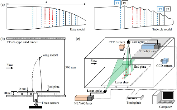
Figure 1. Wing models and experimental setup: (a) planform views of the base and tubercle models; (b) force measurement setup; (c) two-dimensional PIV setup. PIV measurements are conducted at the locations of T1–T7 (troughs) and P1–P7 (peaks). Red dots denote locations of pressure tabs.
Download figure:
Standard image High-resolution imageFigure 1(b) shows the schematic diagram of the force measurement. To minimize the effect of the incoming boundary layer from the wind tunnel floor, an end plate is installed at the test section. The leading-edge of the end plate is shaped into a half ellipse with a ratio of major to minor axis of 2. To reduce leakage flow, the wing models are mounted within 2 mm from the upper surface of end plate, which is within the range of the suggested maximum gap of 0.005 × model span length (Barlow et al 1999). The lift (L) and drag (D) forces on the wing models are measured with force sensors (AND LCB03 series) which are attached to the supporter assembled with the models. Signals from the force sensor are sampled for 60 s at a rate of 10 kHz to obtain a fully converged mean force and digitized by the A/D converter (NI PCI-6259). The lift (CL) and drag (CD) coefficients are defined as CL = L/(0.5ρ A) and CD = D/(0.5ρ
 A), respectively, where ρ is the air density and U∞ is the free-stream velocity. The force measurements are conducted at Re = U∞
 /ν = 180 000, where ν is the kinematic viscosity of air. The angle of attack is varied from 0° to 25° by increments of 1°. Using the method in Coleman and Steele (2009), uncertainties of the measured lift and drag coefficients are estimated to be less than 2.5%.
The velocity fields around the wing models are measured using a 2D-PIV system shown in figure 1(c). The 2D-PIV system consists of a fog generator (SAFEX), a double-pulsed Nd:YAG laser (Litron Lasers) operating at 135 mJ, a CCD camera (Vieworks VH-4M) with a 2048 pixel × 2048 pixel resolution, and a timing hub (Integrated Design Tools). The fog generator produces liquid droplets having a mean diameter of 1 µm, which are introduced into the wind tunnel. Laser and laser optics make laser sheets having a thickness of 2 mm, which illuminate the planes of interest. The x, y, z denote the streamwise, spanwise and vertical directions, respectively. The origin is located 0.48 downstream from the leading-edge of the root plane along the chord line. The velocity measurements are performed on several streamwise (x-z) planes indicated as black solid and blue dashed lines in figure 1(a), and on cross-flow (y-z) planes. An iterative cross-correlation analysis is implemented with an initial interrogation window size of 64 pixel × 64 pixel and a final interrogation window size of 32 pixel × 32 pixel. The interrogation window is overlapped by 50%, leading to spatial resolutions of 0.0086cl (cl: local chord length) on the x-z plane and 0.0048
 on the y-z plane. For selected y-z planes in the pre-stall region, a 2D-PIV is conducted using a reduced field of view. In this case, a final interrogation window size is 16 pixel × 16 pixel and overlapped by 50%, leading to a spatial resolution of 0.000 85
 . One thousand pairs of images are taken to obtain the time-averaged flow field. The uncertainties of velocity and vorticity are estimated to be less than 5.8% and 6.4%, respectively (Willert and Gharib 1991, Fouras and Soria 1998, Raffel et al 2013).
To measure the pressure on the suction surfaces of wing models, we install a total number of 45 pressure taps along the chordwise direction from the leading-edge (0 to 0.6cl with increments of 0.05cl, 0.7cl and 0.8cl) at three spanwise locations of P2, T3 and P3 for the base and tubercle models, respectively (see red dots in figure 1(a)). Pressure tabs are connected to a digital manometer (MKS-220DD) having a measurement range of 0–100 Torr. Signals from the digital manometer are sampled for 40 s at a rate of 10 kHz to obtain a fully converged mean surface pressure and digitized by the A/D converter (NI PCI-6259). The pressure coefficient is defined as  , where P is the time-averaged surface pressure and P∞ is the static pressure at the free-stream.
Surface-oil-flow visualizations are also conducted using a mixture of oil and white dye to obtain flow patterns on the suction surfaces. For the visualization, the wing models are installed horizontally to reduce the oil movement by gravity. Photographs are taken after 180 s to obtain images of fully evolved surface-oil-flow patterns. Videos are also taken to analyse the oil movement in time.
3. Lift and drag forces
Figure 2 shows the variations of the lift and drag coefficients and lift-to-drag ratio with the angle of attack for the base and tubercle models at Re = 180 000, together with the results of Miklosovic et al (2004) at Re = 505 000–520 000. The lift coefficients of both models linearly increase until α = 7° but with slightly different slopes (dCL/dα = 4.87 and 4.58 for the base and tubercle models, respectively). This difference in the slopes was not observed in Miklosovic et al (2004) but was reported in Stanway (2008) who conducted an experiment at lower Reynolds numbers of Re = 44 648–119 060, indicating that the slope difference occurs due to relatively lower Reynolds number considered. The base model stalls at α = 8°, at which the maximum lift coefficient is 0.70. With further increase in α, the lift coefficient rapidly decreases, reaches minimum at α = 13° and then increases again. On the other hand, with tubercles, the lift coefficient increases until α = 11°, maintains roughly a constant value (0.82–0.86) at 11° ⩽ α ⩽ 15°. The stall occurs at α = 15°, and then the lift coefficient decreases with increasing α. At α ⩾ 23°, the lift coefficients of both models are the same, indicating that the tubercles do not play any role at these very high angles of attack. The tubercles delay the stall angle by 7° and increase the maximum lift coefficient by about 22%. The drag coefficient with tubercles is much lower at 9° ⩽ α ⩽ 15° than that of base model (figure 2(b)). The drag coefficients are higher than those of Miklosovic et al (2004) due to lower Reynolds number considered in the present study. With tubercles, maximum lift-to-drag ratio occurs at α = 5°, whereas it does at α = 8° for the base model (figure 2(c)). At higher angles of attack, L/D with tubercles decreases much more slowly and thus is higher than that of base model.

Figure 2. Variations of the force coefficients and lift-to-drag ratio with the angle of attack for the base and tubercle models: (a) lift coefficient; (b) drag coefficient; (c) lift-to-drag ratio.
Download figure:
Standard image High-resolution imageAs explained in section 1, the lift characteristics on a tapered back-swept wing model considered by Bolzon et al (2017a) were very different from the present ones, probably because the taper ratio of the former study, 0.4, was much bigger than that of the present study (about 0.16). On the other hand, for a cambered back-swept wing model with a larger taper ratio of 0.33 by Wei et al (2018a), the lift characteristics are quite similar to the present ones. These results indicated that the taper ratio and camber of 3D wings are important parameters to determine the lift characteristics by tubercles.
4. Flow fields at different angles of attack
4.1. Surface-oil-flow visualizations
Figure 3 shows flow patterns on the suction surfaces of the base and tubercle models using surface-oil-flow visualizations, where the spanwise locations of troughs (T) and peaks (P) are indicated on the top of this figure. Figure 4 shows enlarged views of separation bubbles existing in the P2–P3 region (indicated by blue dashed rectangles in figure 3) for the tubercle model. For the base model, flow separates and reattaches on the suction surface at α = 4°, forming a separation bubble elongated along the spanwise direction (0.43 < y/ < 4.43), as shown in figure 3(a) (also observed by Bolzon et al (2017b) and Wei et al (2018a, 2018b)). On the other hand, in the tubercle model, complex flow patterns are observed in the downstream of tubercles, while a flow pattern similar to that of the base model is maintained in the spanwise location of smooth leading-edge (figure 3(b)). Surface-oil-flow pattern in figures 3(b) and 4(a) shows hemi-spherical separation bubbles right after tubercle troughs. Inside this separation bubble, counter-rotating foci are observed (x/
 ≈ −0.2) (Wei et al 2018a). At a further downstream location (x/
 ≈ 0.1), foci with clockwise and counter-clockwise rotating motions are formed at the spanwise locations between peaks and troughs. The discrete distribution of hemi-spherical separation bubbles near the leading-edge in the tubercle model is similar to that observed from previous studies on 2D airfoil models (Karthikeyan et al 2014, Rostamzadeh et al 2016) and 3D back-swept wing models (Wei et al 2018a, 2018b), although the detailed flow patterns are not precisely matched.

Figure 3. Surface-oil-flow visualizations for the base (left column) and tubercle (right column) models: (a) and (b) α = 4°; (c) and (d) α = 9°; (e) and (f) α = 13°; (g) and (h) α = 16°. Here, the red dashed and solid lines denote the flow separation and reattachment, respectively.
Download figure:
Standard image High-resolution image
Figure 4. Enlarged views of the regions indicated by the blue dashed rectangles in figure 3: (a) α = 4°; (b) α = 9°; (c) α = 13°.
Download figure:
Standard image High-resolution imageAs the angle of attack increases to 9° at which the base model already stalls (figure 3(c)), the tip region of the base model has flow separation without reattachment, but an elongated separation bubble of smaller streamwise size still exists at 0.37 < y/ < 3.13 and further upstream location. Between these two flow regions (i.e. around y/
 = 3.13), a focus with a counter-clockwise rotating motion exists, also denoted as large-scale recirculating region by Wei et al (2018a, 2018b). Moreover, a thin separation bubble (indicated by white line) is newly observed closer to the leading-edge at 2.71 < y/
 < 4.43. For the tubercle model (figures 3(d) and 4(b)), flow separation without reattachment occurs very near the tip region due to its low local Reynolds number (Diebold 2012, Wei et al 2018a), and the focus with a counter-clockwise rotating motion, observed for the base model, occurs near the tip region (at y/
 ≈ 4). On the other hand, flow pattern behind smooth leading-edge is similar to that of the base model. At 1.28 < y/
 < 3.95, hemi-spherical separation bubbles behind the trough become much weaker and smaller and locate further upstream than those for α = 4°, and foci located at the spanwise locations between the peaks and troughs are also much weaker. In addition, flow separates weakly near the trailing edge at the spanwise locations of troughs (figure 4(b)), which is consistent with the observation made by previous studies (Johari et al 2007, Hansen et al 2011, Rostamzadeh et al 2014, Hansen et al 2016, Bolzon et al 2017a, 2017b).
At α = 13° where the lift coefficient of the base model is minimum (figure 3(e)), a thin separation bubble exists near the entire leading-edge (thin white line in this figure), and main flow separation occurs afterwards (red dashed line). Figures 3(a), (c) and (e) clearly indicate that flow separation progresses inboard (i.e. tip to root) as the angle of attack increases (see also Pedro and Kobayashi (2008), Wei et al (2018a, 2018b)). In the tubercle model (figure 3(f)), the separated region near the tip becomes wider than that at α = 9° but is still confined to the outboard. The focus with a counterclockwise rotating motion becomes stronger than that at α = 9° and occupies wider space at y/ ≈ 3.5. Separation bubble still exists behind smooth leading-edge but its streamwise size becomes smaller. Near the trailing edge behind troughs (T1–T4), λ-shaped flow patterns exist, each of which consists of large and small foci with clockwise and counter-clockwise rotating motions, respectively (figure 4(c)). These flow patterns near the trailing edge differ from the delta- or horseshoe-shaped patterns (quasi-symmetric foci with counter-rotating motions) observed from 2D airfoil models (Rostamzadeh et al 2014, Hansen et al 2016).
At α = 16° where the tubercle model already stalls, main separation occurs outboard (y/ > 3.1) and inboard (y/
 < 1.6), and foci with counter-clockwise and clockwise rotating motions exist in between. In addition, hemi-spherical separation bubbles are still observed downstream of troughs (T2–T5), and the λ-shaped flow patterns near the trailing edge now disappear. As illustrated in figures 3 and 4, the hemi-spherical separation bubbles after troughs and λ-shaped surface flow patterns near the trailing edge are the key flow structures of separation delay by tubercles, which are examined from surface pressure and velocity measurements in the following sections.
4.2. Surface pressure measurements
Figure 5 shows the distributions of the surface pressure coefficient at three spanwise locations of P2, T3 and P3 for the base and tubercle models. At α = 4° (figure 5(a)), the surface pressure coefficients of the base model at three spanwise locations are not very different among themselves. The tubercle model, however, shows very different pressure distributions from those of the base model. The peak magnitude of −Cp on the suction surface at the trough T3 is higher than that at the same spanwise location of the base model, while the peak magnitudes at the peaks P2 and P3 are lower than those of the base model. As a result, there is a strong chordwise adverse pressure gradient on the suction surface behind the trough, inducing early flow separation, whereas weaker chordwise adverse pressure gradient is formed behind the peak and thus flow is attached there. Therefore, a hemi-spherical separation bubble is formed behind each trough, as shown in surface-oil-flow visualization (figures 3(b) and 4(a)). At α = 13° (figure 5(b)), the pressure coefficient on the suction surface of the base model is almost flat in the chordwise direction because the flow already fully separates from the suction surface. For the tubercle model, however, the peak magnitudes of −Cp on the suction surface at three spanwise locations are higher than those of the base model because of the separation delay, and strongest adverse pressure gradient is formed in the downstream of the trough T3, which induces strong λ-shaped flow patterns near the trailing edge (figure 4(c)) and nearly flat pressure distribution at x/ > 0.2.

Figure 5. Distributions of the surface pressure coefficient at three spanwise locations of P2, T3 and P3 for the base and tubercle models: (a) α = 4°; (b) α = 13°.
Download figure:
Standard image High-resolution image4.3. Velocity measurements
Figure 6 shows the contours of the instantaneous streamwise vorticity and cross-flow velocity vectors on y-z planes near the trough T3 at three different streamwise locations for the tubercle model at α = 4°. Since flow structures are not clearly visible due to strong attached flow toward the surface, Galilean transformation, adding w/U∞ = 0.12 and 0.2 to the flow fields at x/ = 0.1 and 0.33, respectively, is performed to better identify flow structures (see, e.g. Adrian et al 2000). At x/
 = −0.2 (figure 6(a)), the flow within the hemi-spherical separation bubble does not show distinct flow characteristics but upward flow. At x/
 = 0.1 (figure 6(b)), a counter-rotating streamwise vortex pair evolve from counter-rotating foci inside the hemi-spherical separation bubble. Rostamzadeh et al (2014) observed a similar flow pattern from a 2D airfoil model with tubercles, and Hosseinverdi et al (2015) also found that a streamwise vortex pair evolve from a hemi-spherical separation bubble on a flat plate. As this streamwise vortex pair travel downstream, they move upward due to self-induced motion. An example of such vortex pair is shown in a red dashed box in figure 6(c). Counter-clockwise and clockwise rotating streamwise vortices observed at y/
 ≈ 2.3 and 2.5, respectively, evolve from left and right foci at x/
 ≈ 0.1 (figure 4(a)).
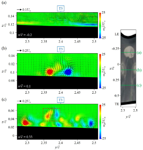
Figure 6. Contours of the instantaneous streamwise vorticity and cross-flow velocity vectors for the tubercle model at α = 4°: (a) x/ = −0.2; (b) x/
 = 0.1; (c) x/
 = 0.33. On the right, the PIV measurement locations are indicated by green lines.
Download figure:
Standard image High-resolution imageFigure 7 shows the contours of the mean streamwise velocity and velocity vectors for the base and tubercle models at α = 9° where the base model already stalls. For the base model, flow separation occurs on P5–P7 planes. Note that separation-reattachment near the leading-edge on P4–P7 planes observed from surface-oil-flow visualization is not measured by PIV owing to low PIV resolution near the surface. For the tubercle model, flow is fully attached on P4–P6 planes and reversal flow is observed near the trailing edge of P7 plane, which is consistent with the results of surface-oil-flow visualization (figure 3(d)). Therefore, flow separation is significantly delayed by tubercles. Figure 8 shows the contours of the instantaneous streamwise vorticity and cross-flow velocity vectors near the trailing edge (at x/ = 0.4) after Galilean transformation (adding v/U∞ = 0.1 and w/U∞ = 0.12 to instantaneous flow fields). Note that the flow fields shown here are measured at different instants owing to the limitation of the size of the field of view. Counter-rotating streamwise vortex pairs are observed in between peak and trough of tubercles, which evolve from foci inside hemi-spherical separation bubbles near the leading-edge as observed at α = 4°. These streamwise vortex pairs prevent the spanwise progression of flow separation from tip to root and delay flow separation at 3.13 < y/
 < 3.95. However, the prevention of spanwise progression was not observed in Wei et al (2018a, 2018b). Due to this difference, the stall delay by tubercles is larger for the present model than for the back-swept wing models in Wei et al (2018a, 2018b).

Figure 7. Contours of the mean streamwise velocity and velocity vectors for the base (left column) and tubercle (right column) models at α = 9°: (a) and (b) P4; (c) and (d) P5; (e) and (f) P6; (g) and (h) P7 planes. Here, the black thick line denotes  = 0. The spanwise locations corresponding to P4–P7are indicated by green solid lines in the upper right figure. Red dots in the upper right figure denote separation points measured by PIV.
Download figure:
Standard image High-resolution image
Figure 8. Contours of the instantaneous streamwise vorticity and cross-flow velocity vectors at x/ = 0.4 for the tubercle model at α = 9°: (a) 3 < y/
 < 3.3; (b) 3.3 < y/
 < 3.6; (c) 3.6 < y/
 < 3.9. On the right, the measurement locations are indicated by green lines.
Download figure:
Standard image High-resolution imageFigure 9 shows the contours of mean streamwise velocity and velocity vectors for the tubercle model at α = 13° where the base model has minimum lift coefficient. In the case of base model, massive flow separation occurs at all spanwise locations. For the tubercle model, flow is attached on most of suction surface. Massive flow separation is observed only on P6 plane (figure 9(e)), and flow separation occurs near the trailing edge only in the downstream locations of troughs (figures 9(a) and (c)). Figure 10 shows the contours of the instantaneous streamwise vorticity and cross-flow velocity vectors on cross-flow planes at three different streamwise locations for the tubercle model at α = 13°. Here, the velocity vectors at x/ = −0.07 are modified through the Galilean transformation by adding w/U∞ = 0.17, to better identify streamwise vortices. At x/
 = −0.07, a counter-rotating streamwise vortex pair appear, similar to those shown at α = 4° (figure 6(b)), which evolve from the hemi-spherical separation bubble in the upstream location. At x/
 = 0.25 (figure 10(b)), a pair of streamwise vortices are observed further away from the surface due to mutual induced motion. Other counter-clockwise and clockwise rotating vortices are found very near the surface (at y/
 ≈ 2.3 and 2.45), which evolve from the upstream foci in the separated flow region (2.28 < y/
 < 2.46). At x/
 = 0.56 (figure 10(c)), streamwise vortices with positive and negative vorticity exist. However, the vortex with negative vorticity is stronger than that with positive vorticity, because the focus with clockwise rotation is stronger than the focus with counter-clockwise rotation (figure 4(c)). Hence, the vortex with positive vorticity moves upward due to the induced flow by the vortex with negative vorticity. It is interesting to note that dominant vortical structure changes from the vortex with positive vorticity to that with negative vorticity as they approach the trailing edge, which is very different from a quasi-symmetric streamwise vortex pair found for 2D airfoil models (Rostamzadeh et al 2014, Hansen et al 2016). These vortical structures delay the stall by suppressing flow separation behind the peaks at α = 13°.

Figure 9. Contours of the mean streamwise velocity and velocity vectors for the tubercle model at α = 13°: (a) T3; (b) P3; (c) T4; (d) T5; (e) P6 planes. Here, the black thick line denotes  = 0. The spanwise locations corresponding to these planes are indicated by green solid lines in the upper right figure. Red dots in the upper right figure denote separation points measured by PIV.
Download figure:
Standard image High-resolution image
Figure 10. Contours of the instantaneous streamwise vorticity and cross-flow velocity vectors for the tubercle model at α = 13°: (a) x/ = −0.07; (b) x/
 = 0.25; (c) x/
 = 0.56. On the right, the measurement locations are indicated by green lines. Note that the scales of the horizontal and vertical axes in (a) and (b) are different from that in (c).
Download figure:
Standard image High-resolution imageFigures 11 and 12 show the flow fields around the tubercle model at α = 16° at which the tubercle model already stalls. At this angle of attack, flow separation occurs near the leading-edge on P1 and P5 planes, but flow is attached at other locations (see also figure 3(h)). As shown from surface-oil-flow visualization (figure 3(h)), foci with clockwise and counter-clockwise rotations exist before the trailing edge. Thus, streamwise vortices with opposite directions of rotation are observed on the cross-flow plane near the trailing edge (figure 12). These two streamwise vortices generate downwash motions towards mid-span surface, resulting in the attached flow there. Although the tubercle model already stalls at this angle of attack, the lift coefficient is still higher than that of the base model because of the attached flow at the mid-span.

Figure 11. Contours of the mean streamwise velocity and velocity vectors for the tubercle model at α = 16°: (a) P1; (b) P2; (c) T3; (d) T4; (e) P4; (f) P5 planes. Here, the black thick line denotes  = 0. The spanwise locations corresponding to these planes are indicated by green solid lines in the upper right figure. Red dots in the upper right figure denote separation points measured by PIV.
Download figure:
Standard image High-resolution image
Figure 12. Contours of the instantaneous streamwise vorticity and cross-flow velocity vectors for the tubercle model (α = 16°): (a) 1.32 < y/ < 1.88; (b) 2.91 < y/
 < 3.47. On the right, the measurement locations are indicated by green lines.
Download figure:
Standard image High-resolution image5. Further discussions
In this section, we compare the role of tubercles on the present 3D wing model with that on 2D airfoil models, and also discuss the effect of tubercles located on the wing root region. In the case of 2D airfoil models without tubercles, main flow separation first occurs near the trailing edge, and moves upstream as the angle of attack increases (Johari et al 2007, Rostamzadeh et al 2014). For the present 3D tapered wing model without tubercles, however, main flow separation first occurs near the tip, and progresses inboard with increasing angle of attack as shown in figure 3, which is consistent with the numerical simulation by Pedro and Kobayashi (2008). The present vortical structures look similar to those of 2D airfoil models with tubercles, but their effects are quite different. In case of 2D airfoil models with tubercles, counter-rotating streamwise vortices evolving from hemi-spherical separation bubbles lead to flow separation near the trailing edge at the spanwise locations of troughs, resulting in degraded performance in the pre-stall region (Rostamzadeh et al 2014). However, in the post-stall region, they induce high momentum near the surface and result in the attached and separated flows behind peaks and troughs, respectively, while the flow fully separates over the base 2D airfoil (Johari et al 2007, Favier et al 2012, Zhang et al 2014). In the case of 3D tapered wing model, in the pre-stall region, streamwise vortices also evolve from hemi-spherical separation bubbles and produce flow separation near the trailing edge due to their induced upward motion behind the trough, which decreases the lift. However, these streamwise vortices prevent the inboard progression of flow separation near the tip region, which compensates the lift loss caused by flow separation near the trailing edge. Previous studies on 3D wing models with a rectangular planform geometry showed that the lift is indeed decreased by tubercles in the pre-stall region (Hansen et al 2010, Yoon et al 2011).
To investigate the effects of smooth leading-edge in the root region for the present tubercle model, another tubercle model (named tubercle model II) is constructed: from root to P1 (0 ⩽ y/ ⩽ 1.71), we add new tubercles which have the amplitude of 0.036cl (nearly the same as the amplitude of P1) and the wavelength of 0.4
 (similar to the wavelength of first tubercle). Figure 13 shows the results from force measurements. The lift coefficient of tubercle model II is similar to that of the original tubercle model up to α = 10°. At 11° ⩽ α ⩽ 15°, the lift coefficient of tubercle model II is slightly lower than that of the tubercle model. In the post-stall region (α ⩾ 16°), however, the tubercle model II has a higher lift coefficient than the original tubercle model because of wider attached region near the root (see below). The tubercle model II has higher drag and lower L/D in the pre-stall region but has better performances in the post-stall region than the original tubercle model does. Figure 14 shows the surface-oil-flow visualizations for the tubercle model II at α = 13° (near-stall region) and 16° (post-stall region). Surface-oil-flow visualization in the near-stall region (α = 13°; figure 14(a)) indicates that trailing-edge separation occurs even in the root region (0 ⩽ y/
 ⩽ 1.71) because of the leading-edge tubercles near the root, which is very different from the results of the original tubercle model (figure 3(f)). At α = 16°, attached flow region on the tubercle model II becomes wider in the root region than the original tubercle model (figure 3(h)), resulting in higher lift coefficient at the post-stall region.

Figure 13. Variations of the hydrodynamic forces with the angle of attack for the base, tubercle and another tubercle models: (a) lift coefficient; (b) drag coefficient; (c) lift-to-drag ratio.
Download figure:
Standard image High-resolution image
Figure 14. Surface-oil-flow visualizations for the tubercle model II: (a) α = 13°; (b) α = 16°. Here, red dashed line denotes flow separation.
Download figure:
Standard image High-resolution image6. Conclusions
In the present study, we experimentally investigated flow structures responsible for the wing performance enhancements by the leading-edge tubercles. The tubercles delayed the stall angle by 7° and increased the maximum lift coefficient by about 22% at the Reynolds number of 180 000. Flow separation first occurred near the tip region for both wing models. As the angle of attack increases, in case of the base model, flow separation near the tip progressed inboard, resulting in full separation. For the tubercle model, however, the stall was delayed because of two vortical motions. The first was the streamwise vortex pairs evolving from foci inside the hemi-spherical separation bubbles near the leading-edge (see figure 15). At α = 4°, the chordwise surface pressure distribution showed that the peak magnitude of −Cp at the trough is higher than that at the peak (figure 5(a)). This resulted in a strong chordwise adverse pressure gradient at the trough, inducing an early flow separation. Hence, a hemi-spherical separation bubble with counter-rotating foci was formed near the leading-edge behind the trough, which generated a streamwise vortex pair in the downstream. These vortical structures were dominant at low angles of attack and prevented inboard spanwise progression of flow separation (from tip to root). The second was the asymmetric streamwise vortex pairs evolving from foci inside separated regions after the mid-chord region, which were dominant flow structures at near-stall angles of attack (figure 15). A vortex with negative vorticity was more dominant than that with positive vorticity as they approached the trailing edge (figure 10). These structures delayed flow separation at the peak spanwise locations, resulting in the stall delay. At a post-stall angle of attack (α = 16°), flow separation occurred in both inboard and outboard regions inside which clockwise and counter-clockwise rotating foci were formed, respectively (figure 3(h)). Streamwise vortices with negative or positive vorticity evolved from these foci (figure 15), and attached the flow in the mid-span region, resulting in a higher lift coefficient than that of the base model. These three types of vortical structures distinguished by their locations of occurrence were given in figure 15.

Figure 15. Schematic diagram of the mechanisms responsible for the performance enhancements by tubercles at various angles of attack. Red and blue curves denote vortices with positive and negative vorticity, respectively.
Download figure:
Standard image High-resolution image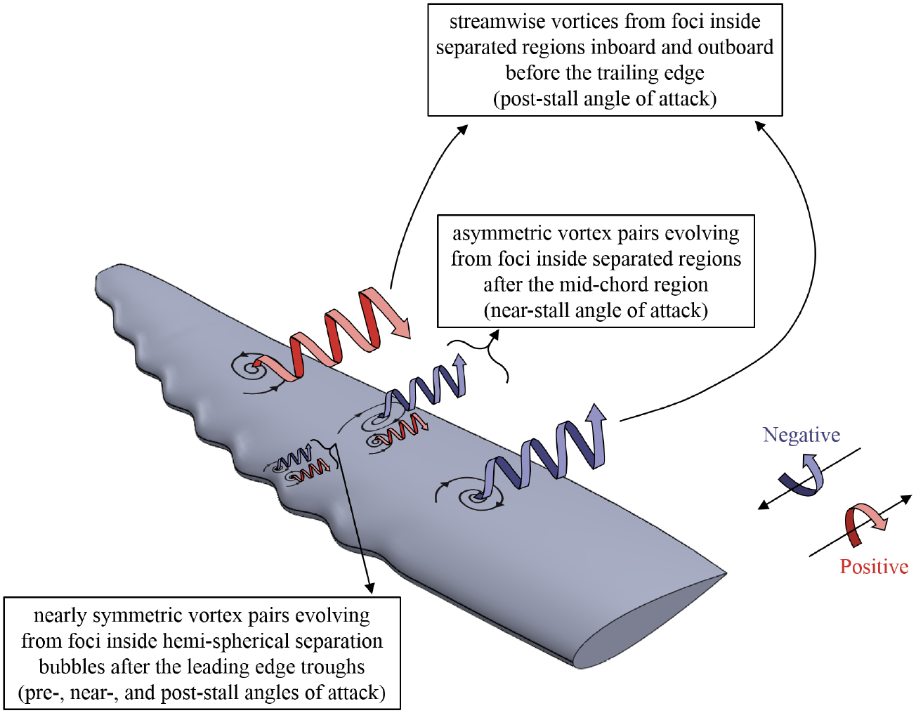
High-speed rotating blades often have high angles of attack at the leading-edge to the incoming flow and contain flow separation there, which degrades the blade efficiency. As they delay separation and increase the lift at high angles of attack, tubercles should be an excellent device for increasing the blade efficiency. Nonetheless, successful applications of tubercles are still limited in engineering (see, for example, Dewar et al (2013) and Choi et al (2015)). The reason for this slow progress is that, as mentioned in section 1, the performance of tubercles notably depends on the wing specifications (such as the wing cross-sectional shape, sweep angle and taper ratio) as well as the Reynolds number, and our current knowledge is still not deep enough to provide optimal tubercle configuration (size and spacing) for a 3D wing. In other words, it is known how the vortical structures above the wing suction side are modified by tubercles (as done in the present study), whereas it is still not known how to choose the tubercle configuration for the best performance of a 3D wing. Thus, a parametric study is always required to find the proper size and spacing of tubercles in engineering phase. To avoid future parametric studies, a systematic study of the tubercle size and spacing should be performed for a wide range of wings (including cross-sectional shapes, sweep angles and taper ratios) and provide tubercle design guidelines.
Acknowledgments
This work was supported by the National Research Foundation through the Ministry of Science and ICT (2016R1E1A1A02921549 and 2014M3C1B1033980).