

Abstract
Inspired by the locomotive advantages that an articulated spine enables in quadrupedal animals, we explore and quantify the energetic effect that an articulated spine has in legged robots. We compare two model instances of a conceptual planar quadruped: one with a traditional rigid main body and one with an articulated main body with an actuated spinal joint. Both models feature four distinct legs, series elastic actuation, distributed mass in all body segments, and limits on actuator torque and speed. Using optimal control to find the energetically optimal joint trajectories, actuator inputs, and footfall timing, we examine and compare the positive mechanical work cost of transport of both models across multiple gaits and speeds. Our results show that an articulated spine increases the maximum possible speed and improves the locomotor economy at higher velocities, especially for asymmetrical gaits. The driving factors for these improvements are the same mechanistic effects that facilitate asymmetrical gaits in nature: improved leg recirculation, elastic energy storage in the spine, and enlarged stride lengths.
Export citation and abstract BibTeX RIS
1. Introduction
Being able to move in an energetically economical fashion is an important requirement for robots and animals alike [1–8]. In nature, energy in the form of food can be a scarce resource. Especially for cursorial animals, this creates a strong incentive to locomote in an efficient manner. Similar constraints apply to robots. Once they have been deployed for a mission in the field, autonomous robots typically do not have many opportunities to recharge their batteries. At the same time, such robots—and in particular legged robots—have only a limited capacity to carry batteries and other fuel sources. To achieve truly autonomous operation, conserving energy is imperative.
It has been shown that legged animals can achieve this economical motion partly by moving in ways that are effectively tuned to their natural mechanical dynamics [9–12]. That is, animals and humans take advantage of movement that arises through the passive interplay of gravity, ground contact forces, the elasticity in their muscles and tendons, and the mechanical inertia in their body segments. Using these natural dynamic motions allows them to store and recover mechanical energy and reduce the active work done by their muscles. Animals exploit, for example, the mechanical dynamics of an inverted pendulum as they walk with relatively straight legs [12]. When humans switch to running, they utilize the compliance in their tendons and muscles to store energy elastically while using a motion that exploits the mechanical dynamics of a spring loaded inverted pendulum [13]. Over the past years, these concepts have been steadily adapted into the world of legged robotics [14], and a number of robotic prototypes have been built that seek to take advantage of similar natural mechanical dynamics to achieve economical locomotion [15–19].
This exploitation of the natural mechanical dynamics has interesting implications for the design of robotic systems. The desire to move economically inherently couples the motion of a legged system to its morphology: the mechanical dynamics that a legged system exhibits are a direct consequence of the way it is built and these dynamics, in turn, dominate the way that an animal or robot should move in order to be economical. In this paper, we investigate a particular aspect of morphology and its potential usefulness in robotics: the articulation in the spine of quadrupeds.
In nature, the advantages of an articulated spine seem to be closely coupled to the choice of gait. At lower speeds, quadrupedal mammals generally utilize symmetrical gaits, in which the legs on the left side perform exactly the same motion as the legs on the right, just 180° out of phase. At higher speeds, they tend to transition to asymmetrical gaits, in which the two sides of the animal perform different motions and/or the phase shift differs from 180° [20]. Animals primarily utilize the articulation in their spine for these high speed asymmetrical gaits [21], whereas less spine motion can be observed in the symmetrical gaits [20]. This is an important observation and any investigation of the usefulness of an articulated spine in legged robots should thus incorporate the question of gait as a key factor in its analysis.
It has been argued that, with an asymmetrical gait, an articulated spine provides a number of dynamical benefits for animals with regard to leg recirculation, elastic energy storage, and stride length. In particular [22], pointed out that the articulation in the spine allows for faster recirculation of the legs. That is, the spinal rotation that is added in series to the flexion and extension of the hip and shoulder joints, enables a faster motion of the legs during swing. He further hypothesized that these additional degrees of freedom allow for longer stride lengths, attributing to a cheetah's high maximum speed [23]. Alexander [20] built upon Hildebrand's hypothesis when examining various models of quadrupedal animals and suggested that muscles and tendons in the articulation of the spine might act as additional elastic elements to store and release energy.
A number of studies have tried to assess the potential benefits of an articulated spine by performing comparative studies among quadrupedal models. Zhao et al [24], for example, developed a pneumatic-driven robotic quadruped with a rigid, passive, and active spine configuration. Using a step-function control pattern to achieve a bounding gait, they found that when the spinal motions are synchronized with leg movements, the extension and flexion of the active spine allows the robot to reach higher speeds. Kani and Ahmadabadi [25] used a central pattern generator controller to obtain bounding gaits for a robotic simulation comparing rigid, passive articulated, and active articulated spinal configurations. They found that bounding with a series elastic actuated spine performed better than an articulated passive spine and rigid spine in terms of bounding power consumption. Haueisen [26] compared two 2D quadrupedal bounding models, one with an articulated spine modeled as 6 rigid segments and one with a rigid spine modeled as 5 rigid segments. With these models, Haueisen analyzed the effects of speed and stride frequency on the energy requirements of both models for the bounding gait. She found that, during bounding, the articulated model utilized its articulated spinal joint in similar ways to that observed in nature and also found energetic benefits at higher speeds. Using optimal control Cao and Poulakakis [27], found that, at sufficiently high speeds, an articulated model of a bounding quadruped was more economical than a rigid model. All of these prior comparative simulation studies considered simplified quadrupedal models that represented a two-legged planar bounding robot. The comparison of the two morphologies has also been explored for bounding in hardware [28], where, in contrast to the above studies, they did not observe an energetic improvement for the flexible spine.
To extend these comparison studies beyond bounding, in this work, our model incorporates four independent legs. This design choice allows us to explore the effect of an articulated spine over the full range of quadrupedal gaits found in nature. This is an important extension, as bounding rarely appears as the gait of choice [29], while other gaits such as walking, trotting, tölting, and galloping are employed by a significant number of quadrupeds of all sizes [30]. Furthermore, our prior work has shown that bounding was never the most economical gait for robots [8]. In addition to the four legs, our model incorporates complexities such as feet with mass, inertia in the legs and torso, detailed motor models with realistic limitations on torque and speed, as well as series elastic springs with damping that generate the rich natural mechanical dynamics necessary for efficient locomotion. These complexities allow for physically realistic motions across a wide range of velocities and gaits.
Utilizing this model, in this paper we investigate whether and how the benefits of an articulated spine translate from nature into the world of robotics. We consider the choice of gait and investigate the three mechanical mechanisms stated above. Our tool of choice for this investigation is physics based simulation which we use to compare two model instances—one with and one without an articulated spine. The coupling of motion and morphology poses a particular challenge in this context: in order to optimally exploit their respective natural dynamics, each of the two morphologies will require distinctly different actuation patterns and joint movements to move forward in an economical fashion. Using the same control strategy for both morphologies would implicitly bias the comparison to favor one or the other. To overcome this issue, we let a numerical optimizer find the best possible joint trajectories, actuator inputs, and footfall timing to minimize the energetic cost of locomotion. By doing this individually for each morphology, we effectively remove the question of control from the comparison. This approach reduces the investigation of the benefits of an articulated spine solely to the mechanical differences between the two model instances. In the process, we create a causal relationship between morphology and performance. In addition to understanding the potential benefits of an articulated spine for robots, this approach also allows us to add new insight into the hypotheses put forth by Hildebrand and Alexander [20, 22, 23].
The dimensions and parameters of our model are roughly based off the quadrupedal robot, StarlETH [31, 32], and are similar to the models used in our previous studies on robotic gait selection [8, 33]. We created two model instances: one with a rigid main body and one with an articulated main body composed of two rigid segments connected by a rotational joint (figure 1). Similar to our previous work [8], we used optimal control to generate an energy cost landscape as a function of speed, using positive mechanical motor work normalized per distance traveled as the cost function. This was done for both model instances across a broad range of different gaits to allow for a fair comparison of the two morphological instances.
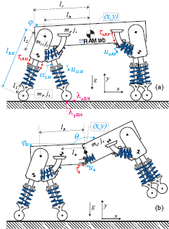
Figure 1. In this work, we investigate the benefits of an articulated spine for the use in quadrupedal robots. We base our comparison on two physics based models: one with a rigid main body (a) and one with an articulated main body (b). Both model instances have four distinct legs and incorporate complexities such as mass and inertia in all body segments, detailed motor models with limits on available torque and speed, as well as series elastic actuators. To ensure that we are making a fair comparison, we use optimal control to find the most energetically economical joint trajectories, actuator inputs, and footfall timing for each model across a broad range of gaits and locomotion velocities.
Download figure:
Standard image High-resolution image2. Methods
In this study, we compare two different instances of a physics-based model of a quadrupedal legged robot: one with a rigid spine (figure 1(a)) and one with an articulated spine (figure 1(b)). We employ optimal control to identify the most economical motion for each of the two instances across a wide range of locomotion speeds and gaits, generating a lower bound on the energetic cost of locomotion. As the model and optimization methods used in this study are similar to the ones used in our previous work [8], we restate them only briefly while focusing on the aspects most critical to the comparison of the rigid versus articulated spine.
2.1. Model
The model is planar and consists of a main body and four individual legs with index  (labeled as left L, right R, hind H, and front F). Its geometrical dimensions are shown in figure 1. The individual segments of the model all have distributed masses with associated inertias. Each leg consists of an upper (m2, j2) and lower (m3, j3) segment that are connected with a prismatic joint that yields a variable leg length of li. The upper leg segments are attached to a main body at hip/shoulder joints (with joint angles
  ) at a distance lr from the center of mass (COM). The main body is either a single rigid segment with mass mr and inertia jr or—in the case of the articulated spine—consists of two identical segments of half the size with mass
  and inertia
  . These two segments are connected with a rotational joint with joint angle θ. The COM of each segment is a distance la from this rotational joint. The position of the center of the main body is given by horizontal and vertical positions x and y, and by the orientation of the main body φ. For the articulated model, we use the orientation of the hind segment
  for the same purpose.
There are three different joint types with index  for leg extension, hip rotation, and spine rotation. All actuators are modelled as series elastic actuators (SEAs) [34], as they were used in our existing robotic hardware [35, 36]. Comparable to ligaments in nature, the series springs give the robot the opportunity to elastically store and release energy in all joints. Each joint is therefore modelled to consist of a spring with stiffness kp and damping coefficient bp that connects to the joint at its distal end while its proximal end is connected to an electrical DC motor and gearbox with reflected inertia
  . For leg extension, this gearbox also converts the motor rotation into a linear motion.
For clarity, we will omit the indices i and p in the following description of the actuators. The position of an actuator (after the gearbox) is given by u and its speed by  . The torque after the gearbox is given by T
In the SEAs, the joint torques/forces F are ultimately produced by the springs according to:
With this, the generalized coordinate vector is given by  for the rigid model and by
  for the articulated model. The vector of generalized torques is given by
  and
and  , respectively.
All model parameters are provided in table 1. The parameters used, including mass, inertia, length, and spring stiffness, are based on our existing hardware [36]. This also holds for the motor/gearbox parameters, such as the reflected inertia  , the maximum output torque
  limitation, and the speed limitation
  . To reduce the number of free parameters, all values have been normalized with respect to total mass mo, uncompressed leg length lo, and gravity g.
Table 1. List of all model parameters. Values are expressed with respect to total mass mo, leg length lo, and gravity g.
| Common properties: | |||
|---|---|---|---|
| m2 = 0.05 mo | m3 = 0.025 mo | j2 = 0.001  |
j3 = 0.001  |
bl = 0.14  |
 = 1.796 mo = 1.796 mo |
 = 0.09 = 0.09  |
lh = 0.75 lo |
| l2 = 0.25 lo |  = 0.449 = 0.449  |
rfoot = 0.05 lo | kl = 5.0  |
| l3 = 0.25 lo |  = 2.5 = 2.5  |
 = 0.79 = 0.79  |
 = 0.15 = 0.15  |
 = 1.360 mog = 1.360 mog |
 = 0.680 = 0.680  |
 = 8.49 = 8.49  |
 = 4.24 = 4.24  |
| Rigid model: | |||
| mr = 0.7 mo | jr = 0.2  |
lr = 0.93 | |
| Articulated model: | |||
| ma = 0.35 mo | ja = 0.025  |
 = 1.57 = 1.57  |
 = 5 = 5  |
 = 0.680 = 0.680  |
 = 0.24 = 0.24  |
 = 8.49 = 8.49  |
la = 0.5 lr |
 = 0.449 = 0.449  |
|||
The equations of motion (EOMs) for this model are stated in a floating base description using additional contact constraints (as described in detail in [14]). They are expressed as a differential algebraic equation:


with the mass matrix  , the differentiable force vector
  , and the generalized torque vector
  . The algebraic function
  encodes the currently active contact constraints. It ensures that all the feet that are in contact with the ground do not slide or penetrate into the ground. The partial derivative of this function yields the contact Jacobian
  whose transpose maps a vector of contact forces
  into the generalized coordinate space.
The sequence of footfalls that happens during locomotion breaks the simulation into individual phases (with index c) and each phase uses a different contact constraint function  . At the end of each phase c (at time tc) a specific number of feet must get in contact with the ground or leave the ground in order to transition into the next phase c + 1. This requirement is encoded by an event function
  that is evaluated at time tc:

Furthermore, at the end of each phase, a collision might happen and velocities change instantaneously to match the new contact constraints  . This instantaneous change in speed can be computed from:


with  being the vector of impulses associated with the collision. Matlab functions to calculate
  ,
,  ,
,  , and
, and  from equations (3) and (4) are supplied in the supplemental files.
By prescribing a particular sequence of functions  and
and  , we determine the gait of the model. The timing of events
  is left open. With this, we enforced eight different footfall patterns which can be broadly classified into a set of symmetrical and asymmetrical gaits (footfall patterns shown in figure 2). Symmetrical gaits are those 'in which the left and right feet of each pair have equal duty factors and relative phases differing by 0.5' [29]. Equivalently, for these gaits, we only simulate half the stride and mirror it to obtain the second half. Asymmetrical gaits are those that do not meet these criteria. The symmetrical gaits we investigate are four-beat walking, two-beat walking, tölting, and trotting. The asymmetrical gaits we investigate are bounding, grounded bounding, galloping, and gallop bounding. The majority of these gaits were chosen based off of our previous work [8]. Grounded bounding and gallop bounding were included because at high speeds, the optimizer chose phase durations within bounding and galloping that approached these gaits.
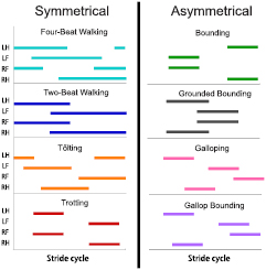
Figure 2. We explored four symmetrical and four asymmetrical gaits, whose footfall patterns are shown in this figure. The colored bars indicate when each leg is in stance (LH: left hind, LF: left front, RF: right front, RH: right hind). While the footfall sequence was fixed, the duration of each phase of the gait, as well as the total stride duration was chosen by the optimizer. The terms two-beat walking, grounded bounding, and gallop bounding were devised by the authors to clearly distinguish these gaits from trotting, bounding, and galloping. Since the models are planar, left and right legs are interchangeable, and some gaits could thus be omitted in our analysis. Pacing, for example, would be indistinguishable from trotting and was hence not considered.
Download figure:
Standard image High-resolution image2.2. Optimization
To compare the energetic economy of both model instances we considered the positive motor work cost of transport (COT). To this end, the positive motor work is computed as the integral of positive mechanical power summed over all motors over the duration of the stride and normalized by total mass and distance traveled:
To improve the numerical behavior, we approximated the discontinuity in the cost function by smoothing the  function using the equation:

with  .
.
With this, we can set up the search for the optimal motion to be a constrained optimization problem, in which we identify optimal joint trajectories  , torque inputs
  , and event times
  :
:

subject to the following constraints:
- The trajectories
 and comply with the dynamics defined in equations (3) and (4).
 - For each phase c, it holds:
- The motion is periodic; i.e. and
- Motor torques, speed, and positions are within the given limits for all joints i and p:
- .
- .
- .
- Vertical foot positions are non-negative, .


This constrained optimization problem was solved through a multiple shooting optimization framework (MUSCOD) (Diehl et al[37]) with methods illustrated and detailed in [8]. We examined locomotion velocities between 0.025  and 4.5
  . For each gait, we conducted an initial optimization at an initial speed and iteratively conducted optimizations at neighboring velocities in a branching method until the full range of velocities was covered or no solutions could be found. In this process, we used previously obtained solutions as the initial conditions of the neighboring velocities. At each particular speed, the solution with the lowest cost was taken as the optimal motion and re-used for re-initialization. This procedure was repeated from a variety of initial seeds to avoid local optima.
3. Results
On average, the optimization of a single gait at a particular speed converged in about 5 minutes on one core of a 2.40 GHz processor. The time it took to process a given gait over the entire range of velocities varied largely. Depending on how well neighboring data points could be used for seeding new runs and on how many data points were recomputed, it took between 2 (trotting) and 28 (gallop-bounding) days to process a gait with the chosen speed resolution.
We found that the articulation in the spine has been used primarily in the asymmetrical gaits. The optimal solutions for the bounding and galloping gaits had large joint motion in the spine, while the spinal joint underwent relatively small deflections over the course of a stride for symmetrical gaits (table 2). An exemplary motion (galloping at  ) is shown for both model instances in figure 3. More representative motions for each gait and model can be found in the supplementary videos (stacks.iop.org/BB/13/036002/mmedia). The resulting cost landscapes are shown in figure 4. Table 3 lists the minimal and maximal speeds for which a solution for each gait was found for each model instance, as well as the average changes in energetic cost and stride length between the two model instances. These averages were computed over the range of speeds at which solutions were found for both model instances and tested for statistical significance.

Figure 3. Video stills of an animation of a full stride of galloping at a speed of  . It is evident that the spinal joint is being used heavily in the articulated model (bottom sequence).
Download figure:
Standard image High-resolution image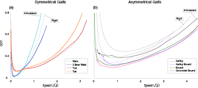
Figure 4. The positive mechanical work cost of transport is shown as a function of forward speed for all gaits that we explored. Solutions for the rigid spine model are presented as dotted lines, and solutions for the articulated spine model as solid lines. For symmetrical gaits, the two models have similar costs (a). For asymmetrical gaits, the articulated model instance has improved energetics and solutions extending to higher speeds.
Download figure:
Standard image High-resolution imageTable 2. Change in spinal angle at a speed of 1.0 .
.
| Gait |  |
|---|---|
| Four-beat walking | 8.04 ° |
| Two-beat walking | 4.14 ° |
| Tölting | 7.83 ° |
| Trotting | 5.20 ° |
| Bounding | 51.5 ° |
| Grounded bounding | 56.4 ° |
| Galloping | 22.4 ° |
| Gallop-bounding | 112.7 ° |
Table 3. Speed range, difference in COT, and difference in stride-length for each investigated gait. p-values are based on a two-sample t-test.
| Gait | Lowest speed |
Highest speed |
Mean COT difference | Mean stride length difference | ||||
|---|---|---|---|---|---|---|---|---|
| Min speed in search: 0.025 | Max speed in search: 4.500 | |||||||
| Rigid | Articulated | Rigid | Articulated | From rigid | p-value | lo From Rigid | p-value | |
| Four-beat walking | 0.025 | 0.081 | 1.644 | 1.925 | 0.078 | <0.001 | 0.257 | <0.001 |
| Two-beat walking | 0.025 | 0.025 | 1.413 | 1.569 | 0.001 | 0.895 | −0.007 | 0.862 |
| Tölting | 0.025 | 0.025 | 3.394 | 3.556 | −0.012 | 0.320 | 0.157 | 0.072 |
| Trotting | 0.025 | 0.025 | 3.294 | 3.306 | 0.004 | 0.578 | 0.110 | 0.386 |
| Bounding | 0.031 | 0.025 | 2.994 | 4.500 | −0.106 | <0.001 | 0.464 | <0.001 |
| Grounded bounding | 0.075 | 0.131 | 4.156 | 4.500 | −0.080 | <0.001 | 0.582 | <0.001 |
| Galloping | 0.094 | 0.106 | 3.338 | 4.500 | −0.034 | <0.001 | 0.316 | <0.001 |
| Gallop bounding | 0.106 | 0.338 | 3.469 | 4.500 | −0.054 | <0.001 | 1.413 | <0.001 |
Among the symmetrical gaits, only four-beat walking showed a significant difference (p < 0.05) between the rigid and articulated models in terms of energetics. Walking with an articulated spine increased energy consumption by 31.8%. All other symmetrical gaits had comparable energetic costs between the rigid and articulated models. Maximal speeds were constrained by the available torque and force capability in the motors. For all symmetrical gaits, the highest speed at which solutions were found was slightly higher for the model instance with the articulated spine.
The benefit of the articulated spine was clearly visible for the asymmetrical gaits, in which the articulation led to improved energetic economy and higher maximal speeds. Table 3 shows that the articulated model was significantly more economical than the rigid model for all asymmetrical gaits. Furthermore, for all asymmetrical gaits on the articulated model, we found solutions all the way to the upper bound of the speed range that we investigated (4.5  ). For the rigid model, in contrast, the maximal speed was constrained to lower values (<4.2
  ) for all gaits, as the motors ran into torque limits. These torque limits were usually reached by the leg extension motors during the stance phase and by the hip motors during the swing phase preempting a particular leg's stance phase. Motor speed limits were generally not reached.
Confirming the results from our previous work [8], the combined cost landscapes showed that minimizing energy cost required switching from gait to gait as speed varies (figure 5). This choice of gait was slightly different for the two model instances. The rigid instance went from four-beat walking at low speeds, to trotting at intermediate speeds, to galloping at high speeds, to grounded bounding at the highest speeds. The articulated instance had the same gait sequence at low, intermediate, and high speeds, but transitioned to gallop bounding at the highest speeds. The biggest difference between the two model instances was observed for the transition speed between trotting and galloping. In particular, the results of the rigid (articulated) model instance indicated a transition from four-beat walking to trotting at a speed of 0.60 (0.53
(0.53 ) and from trotting to galloping at a speed of 2.05
 (1.28
(1.28 ). The rigid instance transitioned from galloping to grounded bounding at a speed of 3.34
 and the articulated instance transitioned from galloping to gallop bounding at a speed of 3.63
 .
.
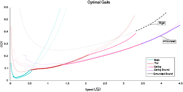
Figure 5. The optimal gait choice for each model instance is shown as a function of forward speed. Rigid solutions are presented as dotted lines, and articulated solutions are shown as solid lines. For clarity, the most economical gait choice at each speed is highlighted. At low speeds, where walking and trotting are the most energetically favorable gaits, the two model instances have similar costs. At higher speeds, where galloping, gallop-bounding, and grounded bounding are the most energetically favorable gaits, the articulated model instance has a much lower COT.
Download figure:
Standard image High-resolution imageTo further investigate the source of the energetic improvements, we focused on the energetic breakdown for galloping (figure 6). Similar results were observed for the other asymmetrical gaits. At a speed of 3.34 , the maximum speed at which we were able to find a rigid galloping solution, the rigid model had a mechanical COT of 0.390 and the articulated model had a COT of 0.284 (Note that the COT, which represents the energy consumed divided by the robot weight and distance traveled (section 2.2), is a unitless quantity). For both models, collisions were the smallest source of losses. At this speed, collision losses accounted for 0.041 of the losses for the rigid model, and for 0.034 of the losses for the articulated model. Damping losses contributed approximately equally to the COT for both models: 0.187 for the rigid model and 0.182 for the articulated model. With these losses being similar, the difference in energetic cost was thus driven primarily by negative motor work. Starting at a speed of around 1.5
 , the negative motor work in the rigid model instance increased relative to the articulated model instance, coinciding directly with the worsened energetic economy of rigid galloping. At a speed of 3.34
 , for the rigid model, negative work accounted for a partial COT of 0.162 and for the articulated model for a partial COT of 0.068.
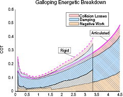
Figure 6. Breakdown of energy losses during galloping as a function of speed. For both model instances, collision losses play only a minor role. Damping losses are comparable for the two instances. The primary difference is an increase in negative work by the rigid model instance relative to the articulated model instance, beginning at a speed of around 1.5 .
.
Download figure:
Standard image High-resolution imageThe primary source of this increased negative motor work were the hip motors used in leg recirculation (figure 7). At a speed of 3.34 , the hips performed 0.154 of the total negative motor work for the rigid model, while only performing 0.033 of the total negative motor work for the articulated model. At that same speed, the legs performed 0.008 of the total negative motor work for the rigid instance and 0.007 of the total negative motor work for the articulated instance. For the articulated model, the motor at the spine performed 0.028 of the total negative work.
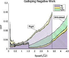
Figure 7. Breakdown of negative motor work during galloping as a function of speed. The negative work performed by the leg motors is comparable for both model instances. At high speeds, the motors at the hips perform much more negative work for the rigid model instance, driving up the overall costs. The articulated model's spinal motor performs additional negative work, but the overall total is still considerably lower than the rigid instance at high speeds.
Download figure:
Standard image High-resolution imageFor asymmetrical gaits, the articulated model used the spinal joint to perform significant amounts of positive work. Table 4 shows the breakdown of positive work performed by the spinal joint for each asymmetrical gait at its maximum speed. It shows the total positive work done by the spinal joint, the portion done actively by the motor, the portion performed passively by the spring, and the portion done by the reflected motor inertia. Note that because the quadrupedal model is not energetically conservative, the value for the joint is less than the sum of the motor, spring, and inertia contributions. The spring performs a relatively small proportion of the positive work compared to the motor and inertia. It is not used to store large amounts of energy. This lack of energy storage is true across all speeds. Galloping is shown as an exemplary case in figure 8. The joint produces a much larger amount of positive work than it absorbs negative work.
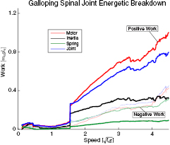
Figure 8. Breakdown of the work performed by the spinal joint during galloping as a function of speed. The positive work is shown as darkly colored lines. The negative work is shown as transparent lines. The joint performs much more positive work than negative work. The spring performs relatively little positive work at all speeds.
Download figure:
Standard image High-resolution imageTable 4. Positive work done at the spinal joint at a speed of 4.5 is broken into contributions by motor, series spring, and rotor inertia. All power values have units of (
 ).
).
| Gait | Joint | Motor | Spring | Inertia |
|---|---|---|---|---|
| Bounding | 0.93 | 1.14 | 0.11 | 0.34 |
| Grounded bounding | 0.66 | 0.93 | 0.11 | 0.30 |
| Galloping | 0.80 | 1.00 | 0.095 | 0.32 |
| Gallop bounding | 0.77 | 1.10 | 0.095 | 0.40 |
Among the symmetrical gaits, only four-beat walking showed a significant difference (p < 0.05) between the rigid and articulated models in terms of stride length. Walking with an articulated spine increased step length by 10.4%. All other symmetrical gaits had comparable stride lengths between the rigid and articulated models. For all asymmetrical gaits the articulated model employed significantly longer stride lengths than the rigid model (table 3).
4. Discussion & conclusion
In this paper, we explored the energetic benefits of including an articulated spine in the torso of a quadrupedal robot. We compared the positive mechanical work COT for two model instances—one with and one without an articulated spine—across multiple gaits and a wide range of locomotion velocities. Using optimal control, we determined the best possible joint trajectories, actuator inputs, and footfall timing to minimize this COT individually for each gait, speed, and model instance. This was done to allow an adaptation of the motion to the respective morphology and to remove the question of control from the comparison. The model that we used built upon the large body of prior work comparing rigid and articulated spines by implementing a number of realistic characteristics, including series elastic actuation, an actuator model with limits on available torques and speeds, and most importantly, four independent legs that allowed us to explore the full range of quadrupedal gaits found in nature.
At higher locomotion velocities (>1.28 ), our comparison revealed large energetic improvements for the articulated spine. In this speed range, asymmetrical gaits (in particular grounded bounding, galloping and gallop bounding) were the most efficient way of locomoting. For the four asymmetrical gaits that we explored, the average savings (within the speed range in which solutions were found for both model instances) were between 17.3% (galloping) and 38.0% (bounding). Furthermore, for the model with the articulated spine, we were able to find solutions at much higher speeds than for the model with the rigid spine, whose maximal speed was limited by the torque limits in the actuators. At lower speeds, symmetrical gaits, in particular four-beat walking and trotting, were optimal. In this speed range, the articulated spine had no positive effect. For symmetrical gaits, the cost values were nearly identical for all gaits. The only exception was four-beat walking with an articulated spine, which was, on average 31.8% more energetically costly than four-beat walking with a rigid spine. Comparing the most economical gaits at each speed, the articulated spine reduced the positive mechanical COT on average by
  across the entire range of velocities.
The benefits of the articulated spine have clearly been a function of the choice of gait. Improvements have primarily been observed for asymmetrical gaits. For symmetrical gaits, the energetic economy was similar for both models. In fact, these symmetrical gaits tend to not use the articulation in the spine and the angle of the spinal joint underwent relatively small changes over the course of a stride (table 2). This is not particularly surprising, since for the symmetrical gaits, the legs of a pair move in opposite directions. That is, any rotation of the spine would only aid one of these legs, while hindering the other. Consequently, the optimizer choose almost no motion in the spine for symmetrical gaits. The same reasoning was put forth by Alexander [20]. He stated that animal energy storage in the longissimus aponeurosis ligament of the spine would not be useful for symmetrical gaits, as in these gaits, 'the left leg of a pair swings forward while the right leg swings back'.
We further found that our robot model benefited from the same mechanistic effects that facilitate asymmetrical gaits in nature: the model exhibited improved leg recirculation, elastic energy storage in the spine, and enlarged stride lengths [20, 22, 23].
4.1. Leg recirculation
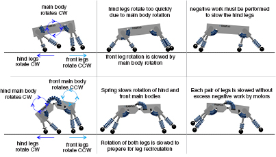
The articulated model's improved leg recirculation manifested itself in two ways: it increased the top speeds that the model was able to achieve (table 3) and it decreased the amount of negative work performed by the motors (figure 6). In the rigid model, the main body can only pitch in one direction. During phases of the gait in which the hind and front legs are moving in opposite directions (e.g. when the hind legs move backwards during stance to push off while the front legs move forwards to extend the stride and prepare for impact), the main body pitch can only aid one of these motions while impeding the other (figure 9). This leads to an increase in work that needs to be done by the hips, and eventually results in an increase in negative work that is done by the hip motors (figure 7). This negative work drives up the mechanical cost of transport for the rigid model. The decoupling of the front and back halves of the torso in the articulated model reduces the negative work done by the hip motors and minimizes the overall energetic cost. It further allowed the articulated model to move its legs quicker without violating torque constraints on the motors; resulting in higher maximal speeds than the rigid model instance. This argument builds upon the hypothesis by Hildebrand [22] about leg recirculation where he states that the flexible spine helps by 'advancing the limbs more rapidly'. Here it is clear that the articulated spine also helps by slowing the limbs without removing excess energy from the system.
Figure 9. The figure shows an annotated version of a typical Galloping gait for both the rigid and articulated model instances at high speeds. For the rigid model (shown in the top row) the main body is only able to rotate in a single direction, moving the hind legs too quickly. As a result, excess negative work is performed by the hips to slow the legs. The articulated model (shown in the bottom row), in contrast, can have each half of the main body rotate, utilizing the spinal spring to slow the legs without performing excess negative work at the hips.
Download figure:
Standard image High-resolution image
4.2. Elastic energy storage in the spine
The articulated model was able to use the spinal spring to store and recover energy (table 4), however, this value was small when compared to other sources of work in the joint. This is a surprising result, as quadrupedal mammals utilize their longissimus aponeurosis tendon to store energy [20]. Still, despite this lack of energy storage, the spinal joint still largely improves energetics. It achieves this improvement by producing a great deal more positive work than negative work (figure 8). That is, the joint is powering the gait by compensating for losses elsewhere. It is possible that a different string stiffness, one that is better tuned to the frequency of spine oscillation, would be more heavily utilized as an energy storage element.
4.3. Enlarged stride length
On average, the model instance with the articulated spine used longer strides than the model with the rigid spine (table 3). This choice of the optimizer, as compared for example to achieving higher speed motions by using the legs at a higher stride frequency, is also in agreement with what was observed in nature [23]. Hildebrand argues that this stride extension happens in concert with the improved leg recirculation. He states that by increasing the swing speed of the limbs, they cover more distance during the swing phase, and extend the duration of the stance phase, leading to longer strides.
Beyond the optimal control based approach, one of the main differences between this study and the existing work was the inclusion of four distinct legs in our model. While past studies have already indicated that a flexible spine is useful for quadrupedal robots, they have all lumped together the two front legs and two hind legs, and could thus only consider a bounding gait [20, 24–27]. Our results support the finding that bounding with the articulated model is more economical than bounding with the rigid model. Yet, bounding was never the most economical gait for the articulated model instance. In fact, it was 6.26 more costly than galloping on average. Having four legs was thus a crucial extension, as it allowed us to explore a broader variety of gaits. Confirming the results of our past work [8], minimizing energetic cost required switching between these different gaits as forward speed increased. The optimal gait sequence differed for the two model instances, but both required distinct motions for all four legs. For the rigid instance, the optimal gait sequence was walking, trotting, galloping, and grounded bounding. For the articulated instance, the optimal gait sequence was walking, trotting, galloping, and gallop bounding. The main difference between the two model instances was that, with the articulated spine, it paid off to switch from trotting to galloping at a much lower speed. This is a direct consequence of the fact that the articulated spine improved only the asymmetrical gaits (galloping) while leaving the energetics of the symmetrical gaits (trotting) unchanged.
Our simulation results strongly suggest that an articulated spinal joint can provide an energetic benefit for legged robots. Yet, before adding a spine to a robotic prototype, additional considerations should be taken into account. The addition of another motor, gearbox, spring, and mechanical joint will add complexity and weight to the robot which has to be compared to the potential energetic benefits. In particular the positive effects of the articulated spine did only manifest themselves at higher speeds, so hardware designers should carefully choose their desired operating speeds before implementing an articulated spinal joint. At low speeds the joint provided no benefit, and for four-beat walking, actually increased costs. In a hardware implementation, it might thus be useful to employ a physical clutch to disable the spinal joint during slow and intermediate velocities, when using symmetrical gaits such as walking and trotting.
It is important to note that it was not a priori given that our optimization based approach would yield the same locomotion strategies that have been observed in nature. The optimizer did not know, for instance, how a typical galloping gait looks. It was not made aware of the differences between symmetrical and asymmetrical gaits and it could have chosen, for example, to not use the motor or spring in the spine or to not increase the articulated model's step length. Still, the optimizer found the exact same gaits to be optimal and discovered the same gait characteristics that are found in nature. For example, similar to quadrupeds in nature, both model instances transitioned from walking to trotting at normalized speeds between 0.5 and 0.7
 [38]. Additionally, many quadrupeds in nature transition from symmetrical to asymmetrical gaits at normalized speeds between 1.4
 and 1.7
 [38]. The rigid and articulated model instances were slightly above and below this range respectively.
While our initial objective was to learn from nature how to build better robots, these findings let us also learn something about nature from robotics. These similarities add strong support to the mechanistic hypotheses that have been used to explain the observed motions of animals. By comparing the best possible motion of each model instance, we essentially removed the question of motion generation and control from the investigation, and our optimization approach thus established a direct causality between the mechanical dynamics of a certain morphology and the resulting motion. Such a causality is almost impossible to establish in comparative biology. In particular, animals have many considerations that can act as confounding factors. These other factors include reducing skeletal stresses [39], improving stability [40], and even predation evasion tactics [41]. For example, a cheetah may utilize its spine heavily at high speeds to facilitate compression of its lungs for oxygen exchange. By using optimization on robotic model instances, we were able to remove such physiological and neurological effects and could focus exclusively on the dynamical advantages of an articulated spine as they have been proposed by Hildebrand and Alexander. Our results seem to verify their hypotheses and highlight the importance of the natural mechanical dynamics in the spine.
Still, it is important to note that our model reflects just one out of many different possible implementations of a quadrupedal robot (see for example [42–45]). In the process of developing the study presented in this paper, we made a substantial number of decisions when selecting model structure, specific model parameters, and the employed cost function. These choices affect the optimal motion. It is likely, for example, that a different morphology would favor different asymmetrical gaits at high speeds. For example, in nature, bounding gaits tend to be preferred by animals with torsos that are relatively long when compared to leg length. These gaits can be particularly useful at high speeds, when the force output of the leg muscles is near saturation, as simultaneous push off of the hind feet provides a greater propulsive force (perhaps indicating why grounded bounding was favored by the rigid model instance at high speeds). Animals with shorter torsos compared to leg lengths, however, tend to prefer galloping gaits [46]. The effect of an articulated spine on gait energetics for these various morphologies is an area ripe for exploration. Still, regardless of the specific morphology, quadrupedal animals generally favor symmetrical gaits at low speeds and asymmetrical gaits at high speeds [46].
Therefore, even with the specific choices that we have made, our results seem to point in a more general direction. Despite the vast differences between our robot model and animals, our results closely resembled what has been observed in nature. These similarities point to fundamental causes for the improved performance with an articulated spine. This also likely means that our results will extend to a wide range of robotic prototypes beyond the specific model considered in this work. Future studies could aim to verify this claim and explore the range of possible parameter values and robot structures. However, we would actually advocate to go one step further and include these properties directly in the optimization. With the development of suitable optimization tools and computational power, this approach would turn the investigation of the benefit of a certain morphology directly into a design process that tells us how a quadrupedal robot should be built.
Acknowledgments
This material is based upon work supported by the National Science Foundation under Grant No. 1453346.