Coalescent processes emerging from large deviations

This paper is organized as follows. In section 2.2 we describe the model under consideration, which is a particular instance of the Cannings model. In sections 2.1 and 2.3 we review some of the background of coalescent theory and review what is known about this model. In section 3 we present our main result, which concerns the limiting coalescent when both the population size and offspring variation are taken to be large. We also discuss the relationship between our results and [CGCSWB22]. Section 4 is devoted to the REM and the connection between our results and the thermodynamic limit of the REM.

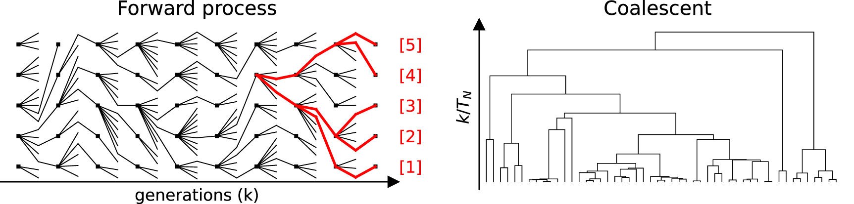
For a realization of the Cannings model with population size N, the corresponding discrete coalescent process on a sample of size n, denoted by $(\Psi_{n,k}^N)_{k\unicode{x2A7E}0}$, describes the genealogical tree obtained by following each sampled individual's ancestors back through time and grouping branches when individuals share a common ancestor. This process is shown in figure 1. We can understand $\Psi_{n,k}^N$ as the state of this tree k generations back from the time our original sample was taken. To define $\Psi_{n,k}^N$ more mathematically, let ${\mathcal{P}}_n$ denote the space of partitions on $[n] = \{1,\dots,n\}$; that is, each element of ${\mathcal{P}}_n$ is a set of disjoint subsets of $[n]$ whose union is $[n]$. Then $\Psi_{n,k}^N$ is a Markov chain taking values in ${\mathcal{P}}_n$ and $\Psi_{n,0}^N$ is the partition into singletons: $\Psi_{n,0}^N = \{\{1\},\{2\},\dots,\{n\}\}$. For k > 0, indices $i,j \in [n]$ are in the same block of the partition if and only if the ith and jth individuals in the original sample share an ancestor k generation in the past.

Zoom In Zoom Out Reset image size

The continuous time coalescent processes which emerge as limits of $\Psi_{n,k}^N$ from any exchangeable Cannings model have been characterized in [MS01]. The authors consider the large-N limit of the time-scaled coalescent process

$$\begin{equation*} \Psi_{n}^N\left(t\right) = \Psi_{n,\lfloor t/c_N\rfloor}^N, \end{equation*}$$

where c_N is the probability that two randomly selected individuals in one generation share an ancestor in the previous generation. Observe that $c_N^{-1}$ is simply the coalescent time, since the number of generations to the most recent common ancestor of two random selected individuals from the current generation follows a geometric distribution with parameter c_N . Recall that $\{\nu_i\}$ are the offspring numbers after resampling the total offspring pool (see equation (1)). The chance that two individuals are both descendants of the first individual in the previous generation is $(\nu_1/N)(\nu_1-1)/(N-1)$. Multiplying by N and averaging over all possible $\{\nu_i\}_{i = 1}^N$ gives

$$\begin{equation} c_N = \frac{\mathbb{E}\left[\nu_1\left(\nu_1-1\right)\right]}{N-1}. \end{equation} \tag{ 2 }$$

We emphasize that, given the distribution of U_i , it is not straightforward to compute c_N because it has a nonlinear dependence on the sum S_N .

The precise notion of convergence considered is in the Skorohod sense ³ – see [EK09] for details. If $(\Psi_n(t))_{t\unicode{x2A7E}0}$ converges to a continuous time process $(\Psi_{n}^N(t))_{t\unicode{x2A7E}0}$ in the Skorohod sense, the possible transitions that can occur in the process $\Psi_n(t)$ involve $\sum_{i = 1}^rk_i$ of the $n = \sum_{i = 1}^rk_i+s$ blocks in ${\mathcal{P}}_n$ merging into r lineages by collapsing into groups of sizes $k_1,\dots,k_r$ while s lineages remain unchanged. Such events are called $(n,k_1,\dots,k_r;s)$ collisions. The rates of these collisions, which uniquely determine the law of $\Psi_{n}(t)$, will be denoted by $\lambda_{n,k_1,\dots,k_r;s}$ for n > 2.

In order to relate the merge rates $\lambda_{n,k_1,\dots,k_r;s}$ to the distribution of ν_i , one notes that after conditioning on $\{\nu_i\}_{i = 1}^{N_{\zeta}}$ the chance that r groups of sizes $k_1,\dots,k_r$ each descended from individuals $1,\dots,r$ in the previous generation is

$$\begin{equation*} \frac{1}{\left(N\right)_{\sum_{i = 1}^rk_i}}\prod_{i = 1}^r\left(\nu_i\right)_{k_i}. \end{equation*}$$

It follows that

$$\begin{equation} \lambda_{n,k_1,\dots,k_r;0} = \lim_{\zeta \to \infty}c_{N}^{-1}N^{r-n}\mathbb{E}\left[\prod_{i = 1}^r\left(\nu_i\right)_{k_i}\right]. \end{equation} \tag{ 3 }$$

In particular, if this limit exists and $c_{N}^{-1}\to \infty$, the time-rescaled coalescent $\Psi_{n}^{N}(t)$ converges to a process $\Psi_{n}(t)$ with merger rates given by equation (3). The rates for s > 0 can be obtained via a certain recursive relation discussed in [Sch01].

Of particular relevance for our results are those coalescent processes for which there are multiple mergers, but not simultaneous multiple mergers—in this case $\lambda_{n,k_1,\dots,k_r,s} = 0$ unless r = 1. Such coalescents are known as Λ-coalescents and are defined by the merger rates

$$\begin{equation} \lambda_{n,k} = \lim_{N \to \infty}c_{N}^{-1}N^{1 - n}\mathbb{E}\left[\left(\nu_1\right)_k\right]. \end{equation} \tag{ 4 }$$

Any rates defined in this way will satisfy the consistency condition

$$\begin{equation} \lambda_{n,k} - \lambda_{n+1,k} = \lambda_{n+1,k+1}, \end{equation} \tag{ 5 }$$

which is proved in [Pit99]. The intuition behind equation (5) is as follows: the difference between the rate to see k mergers in a sample of size n and n + 1 is entirely caused by mergers of k + 1 lineages in the sample of n + 1, since these look like k mergers when restricted to the sample of size n. Pitman also proved that any triangular array $\{\lambda_{n,k}\}_{n = 1,\dots,\infty,k = 1,\dots,n}$ satisfying equation (5) has a representation in terms of a positive measure $\Lambda:[0,1]\to \mathbb{R}_{\unicode{x2A7E}0}$ via the relation

$$\begin{equation} \lambda_{n,k} = \int_0^1 z^{k-2}\left(1-z\right)^{n-k}\Lambda\left({\mathrm{d}}z\right). \end{equation} \tag{ 6 }$$

Thus, there is a correspondence between the coalescent process and positive measures on the unit interval.

A simple criterion for the convergence to a Λ-coalescent is found by noting that if $\lambda_{2,2,2;s} = 0$ then there are no simultaneous multiple mergers, since these would contribute to this rate. Therefore, if $c_N \to 0$ and

$$\begin{equation} \lim_{N \to \infty}c_{N}^{-1}\frac{\mathbb{E}\left[\left(\nu_1\right)_2\left(\nu_2\right)_2\right]}{N^2} = 0, \end{equation} \tag{ 7 }$$

the limit process of the genealogy $(\Psi_{n,k}^{N})_{k\unicode{x2A7E}0}$ is a Λ-coalescent [MS01]. The following proposition, which follows from propositions 1 and 3 of [Sch03], summarizes these observations.

Proposition 1. If $c_{N} \to 0$ and equation (7) is satisfied, then as $N \to \infty$, $(\Psi_n^N(t))_{t\unicode{x2A7E}0} = (\Psi_{n,\lfloor t /c_{N} \rfloor}^{N})_{t\unicode{x2A7E}0}$ converges (in the Skorohod sense) to a Λ-coalescent $(\Psi_{n}(t))_{t\unicode{x2A7E}0}$ with merger rates $\lambda_{n,k}$ given by equation (4) for k = n and equation (5) otherwise.

In order to study the situation where the variation in offspring numbers is finite, but large relative to the population size, we set

$$\begin{equation} U_i = {\mathrm{e}}^{\zeta \Phi_i},\quad i \in \left[N\right] \end{equation} \tag{ 8 }$$

where $\{\Phi_i\}_{i = 1}^N$ are i.i.d. and ζ is a deterministic parameter. Since we are interested in the large noise limit, we will eventually take $\zeta \to \infty$. In the remainder of this paper, in order to avoid ambiguity, we will replace i with 1 when referencing elements of an exchangeable random vector. Note that, technically, U₁ should take values in $\mathbb{Z}$; however, in the large noise limit the distinction is not relevant. Moreover, taking $\zeta \to \infty$ implies $\mathbb{E}[U_1]\to \infty$, so we can assume that

$$\begin{equation} \mathbb{E}\left[U_1\right]>1. \end{equation} \tag{ 9 }$$

Offspring distribution of the form (8) were also considered in [SJHW23] within the context of a model including heritability and [CGCSWB22] in a model of dormancy.

It is biologically sensible to work with variation on an exponential scale whenever the organisms in question proliferate exponentially between bottlenecks. In this context, $\zeta \Phi_i$ is the product of the duration of growth between bottlenecks and the time-averaged growth rate for the offspring of the ith cell. For example, imagine an asexual population that is subject to successive cycles of growth and dilution in a heterogeneous environment. An example is a microbial pathogen, such as Mycobacterium tuberculosis [Gag18, FVJH+21]. Suppose that after passing through a bottleneck, each of the N cells occupies a spatially distinct location. Then, due to heterogeneity in the environment, the offspring of each cell will proliferate at different rates, $\Phi_i$. If ζ is the duration of the growth phase, the total number of offspring from the ith cell (before resampling) will be of the form (8). Alternatively, one could imagine that it is the duration of the growth phase which is random—for example, due to a period of dormancy before growth—while the growth rates are fixed. In this case we would use ζ to denote the growth rates and $\Phi_i$ the duration of the growth phase. Such a dormancy model was studied in [CGCSWB22].

We focus on the case where Φ₁ has a stretched exponential distribution, which essentially means that the large deviations of Φ₁ are scale-invariant. Specifically, let

$$\begin{equation*} W\left(\phi\right) \equiv -\ln P\left(\Phi_1 > \phi\right). \end{equation*}$$

We assume $W(\phi)$ is smooth and bounded as φ → 0 and, inspired by [Eis83, BABM05, RAT15], assume

$$\begin{equation} W\left(\phi\right) \sim W^*\left(\phi\right) \equiv \frac{1}{q}\phi^{q},\quad q\unicode{x2A7E} 1. \end{equation} \tag{ 10 }$$

as $\phi \to \infty$. The pre-factor of $1/q$ is arbitrary, since this can be absorbed into ζ, but this particular form leads to some more elegant analytical formula. Note that we can always set $\mathbb{E}[\Phi_1] = 0$ without loss of generality, since the contribution from ${\mathrm{e}}^{\zeta \mathbb{E}[\Phi_1]}$ cancels in the ratio $U_1/S_N$. Note that offspring distributions satisfying equations (9) and (10) include the special cases where U₁ is exponential $(q = 1)$ and lognormal $(q = 2)$.

We now return to the Cannings model with offspring distributions given by equation (10). When q = 1, $\Phi_i$ has exponential tails and the offspring sizes, U_i , have power law tails

$$\begin{equation} P\left(U_i>u\right) = P\left(\Phi_i >\frac{1}{\zeta}\ln u\right) \sim Cu^{-\alpha_1} \end{equation} \tag{ 11 }$$

for $\alpha_1 = 1/\zeta$ and some constant C > 0. The large N limit of the Cannings model with power law offspring (and ζ fixed) is covered by the main result of [Sch03] and theorem 1.3 of [CGCSWB22], which we have reproduced below in a slightly abbreviated form.

Theorem 1 (Theorem 4 from [Sch03]). Assuming equation (11) holds, then as $N \to \infty$ we have

• When $2 \unicode{x2A7D} \alpha_1$, $\Psi_{n,\lfloor t /c_N \rfloor}^N$ converges to the Λ-coalescent with $\Lambda = \delta$, which is called the Kingman coalescent.
• For $1\unicode{x2A7D}\alpha_1\lt2$, $\Psi_{n,\lfloor t /c_N \rfloor}^N$ converges a Λ-coalescent where Λ given by a β-distribution $\textrm{Beta}(2-\alpha_1,\alpha_1)$. It follows from equation (6) that the merger rates are
  $$\begin{align} \lambda_{n,k} = \frac{B\left(k-\alpha_1,n-k+\alpha_1\right)}{B\left(2-\alpha_1,\alpha_1\right)}, \end{align} \tag{ 12 }$$
  where $B(a,b) = \Gamma(a)\Gamma(b)/\Gamma(a+b)$ is the beta function. This process is called a β-coalescent with parameter α₁.
• For $\alpha_1\lt1$, lineages will coalesce in $O(N^0)$ and hence there is a discrete time limit coalescent. We refer to [Sch03] for a detailed description of this process.

This theorem is closely related to the generalized central limit theorem (GCLT) for the sum S_N —see [Hal18, OH21]. Recall that the GCLT tells us that there are two critical points for the limit law of S_N , one where the central limit theorem (CLT) breaks down (α₁ = 2) and another where the law of large numbers (LLN) breaks down (α₁ = 1), see e.g. [Ami20b, Ami20a, Nol20]. In theorem 1, these critical points correspond to the appearance of multiple mergers and the disappearance of any continuous time limit process, respectively.

Our main result concerns the case where q > 1. We reiterate that in this case the variance is finite for all ζ and, therefore, in the large N limit (with ζ fixed) the convergence is to the Wright–Fisher diffusion for the allele frequencies and Kingman coalescent for the genealogies. For any fixed N, if ζ is large enough the Wright–Fisher diffusion/Kingman models are of course going to provide a very poor approximation. In order to better understand exactly what happens when ζ is large, but finite, we set $N = N_{\zeta}$ where N_ζ grows with ζ in such a way that there is a well-defined limit process as $\zeta \to \infty$. As discussed in section 4, the appropriate scaling is related to the thermodynamic limit of the REM [Eis83, BABM05].

To state our scaling assumption, we define the cumulant generating function,

$$\begin{equation*} r_{\zeta} = \ln \mathbb{E}\left[{\mathrm{e}}^{\zeta \Phi_i}\right]. \end{equation*}$$

To simplify some formulas later on, we define $A_{\zeta} \equiv \mathbb{E}[S_{\zeta}] = N_{\zeta}{\mathrm{e}}^{r_{\zeta}}$ with

$$\begin{equation*} S_{\zeta} \equiv S_{N_{\zeta}} = \sum_{i = 1}^{N_{\zeta}}{\mathrm{e}}^{\zeta \Phi_i}. \end{equation*}$$

The relationship between r_ζ and $W^*(z)$ is crucial for our analysis. Using the Laplace method [DB81], which amounts to evaluating $\mathbb{E}[{\mathrm{e}}^{\zeta \Phi_i}]$ where the integrand attains its maximum, it can be shown that r_ζ is asymptotically the convex conjugates of $W^*$. As a result, these functions are related according to the Legendre transform [Tou05]:

$$\begin{equation*} r_{\zeta} \sim r_{\zeta}^* = \inf_{z \unicode{x2A7E}0}\left\{z \zeta - W^*\left(z\right)\right\}. \end{equation*}$$

It then follows from equation (10) that

$$\begin{equation} r_{\zeta}^* = \frac{1}{q^{^{\prime}}}\zeta^{q^{^{\prime}}}, \end{equation} \tag{ 13 }$$

where q' is the so-called dual exponent $q^{^{\prime}} = q/(q-1)$. The equivalence between equations (13) and (10) is a special case of Kasahara–de Bruijn's exponential Tauberian theorem [Mik99].

It follows from equation (13) that all the moments of U_i grow as $\zeta^{q^{^{\prime}}}$, since

$$\begin{equation*} \mathbb{E}\left[U_i^m\right] = \mathbb{E}\left[{\mathrm{e}}^{m\zeta \Phi}\right] = {\mathrm{e}}^{r_{m\zeta}} \sim {\mathrm{e}}^{m^{q^{^{\prime}}}r_{\zeta}^*},\end{equation*}$$

Intuitively, if $\ln N_{\zeta}$ grows slower than $\zeta^{q^{^{\prime}}}$ then N_ζ cannot keep up with the variation as ζ increases and no continuous time limit process will exist. This serves as motivation for the scaling assumption,

$$\begin{equation} N_{\zeta} = {\mathrm{e}}^{\tau r_{\zeta}}. \end{equation} \tag{ 14 }$$

Here, τ is a control parameter closely related to temperature in the REM. Limit theorems for the sum S_ζ under this scaling assumption are proved in [BABM05]. Much like in the GCLT, S_ζ has two critical points, one where the CLT breaks down and one where the LLN breaks down. Moreover, the limit law of S_ζ is α-stable (see theorem 4 in section 4), which strongly suggests a connection between the limit coalescent processes obtained from offspring distributions of the form (8) under the scaling assumption (14) and those described by theorem 1. We note that sums over random exponentials also appear in statistical applications [LGA20, RAT15, SSO12].

The following theorem generalizes theorem 1 to the case q > 1. Interestingly, we find that the β-coalescent emerges universally from exponentially large offspring variation.

Theorem 2. Assume equations (10) and (14) hold with q > 1. Let

$$\begin{equation} \alpha_{q} = \left(W^*\right)^{^{\prime}}\left(\left(1+\tau\right)r_1^*\right) = \left(\frac{1+\tau}{q^{^{\prime}}}\right)^{q/q^{^{\prime}}}. \end{equation} \tag{ 15 }$$

and $\Psi_{n,k}^{\zeta} = \Psi_{n,k}^{N_{\zeta}}$. Then

• For $1\lt\alpha_q\lt2$, as $\zeta \to \infty$ the discrete coalescent process $(\Psi_{n,\lfloor t /c_{\zeta}\rfloor}^{\zeta})_{t\unicode{x2A7E}0}$ converges to a β-coalescent with parameter α_q .
• For $\alpha_q \gt2$, $(\Psi_{n,\lfloor t /c_{\zeta}\rfloor}^{\zeta})_{t\unicode{x2A7E}0}$ converges to the Kingman coalescent.

In figure 2, the region $1\lt\alpha_q\lt2$ is plotted for various values of q. By moving upwards through these regions, we obtain β-coalescents. As expected, for larger q, the region becomes more tilted towards the right, since a larger value of ζ is needed to obtain a continuous-time limit process for the same N. As q → 1, the region becomes a vertical strip between $1/\zeta = 1$ and $1/\zeta = 2$; hence, theorem 1 is retrieved in this limit. The regime $\alpha_q \unicode{x2A7D} 1$ requires a different treatment not covered by this result, but is closely related to calculations of the Gibbs measure for the REM at low temperature, as we discuss in section 4.

Zoom In Zoom Out Reset image size

We will discuss theorem 2 in section 5. Here, we provide an outline of the derivation that will be useful when making the comparison to results for the REM. Following [Sch03], note that we can replace ν₁ with $NU_1/S_N$ when computing averages (this is justified by lemma 3). Therefore,

$$\begin{equation} \mathbb{E}\left[\left(\nu_1\right)_k\right] \sim \mathbb{E}\left[\nu_1^k\right] \sim N_{\zeta}^k\mathbb{E}\left[\left(\frac{U_1}{S_{\zeta}}\right)^k\right]. \end{equation} \tag{ 16 }$$

An LLN for S_ζ (lemma 2) allows us to replace S_ζ with $U_1 + N_{\zeta}{\mathrm{e}}^{r_{\zeta}}$ (this is justified by lemma 6). Hence, letting $f_U(u)$ denote the density of U_i and replacing sums with integrals (this is justified rigorously by [Sch03, lemma 12]), we have

$$\begin{align} & N_{\zeta}^k\mathbb{E}\left[\left(\frac{U_1}{S_{\zeta}}\right)^k\right] \sim N_{\zeta}^k\int_1^{\infty}\frac{u^k}{\left(u+N{\mathrm{e}}^{r_{\zeta}}\right)^k}f_U\left(u\right)\textrm{d}u \end{align} \tag{ 17 }$$

$$\begin{align} & \quad = {\mathrm{e}}^{r_{\zeta}}N_{\zeta}^{k+1}\int_{\left(A_{\zeta}\right)^{-1}}^{\infty}\frac{z^{k}}{\left(z +1\right)^k}f_U\left(zA_{\zeta}\right)\textrm{d}z. \end{align} \tag{ 18 }$$

To obtain the last equation we have changed variables $z = u/A_{\zeta}$. If f_U is a power law, then the integral can be evaluated and is given in terms of Γ-functions—this is one way to prove theorem 1, although a different approach is taken in [Sch03]. The essence of our argument is that when we evaluate this integral we can replace $f_U(zA_{\zeta})$ with ${\mathrm{e}}^{W^*(\zeta^{-1}(\ln A_{\zeta} z))}$ and then neglect the higher-order terms in

$$\begin{eqnarray*} W^*\left(\frac{\ln A_{\zeta} z}{\zeta}\right) & = W^*\left(\frac{\ln A_{\zeta}}{\zeta}\right) + \frac{1}{\zeta}\left(W^*\right)^{^{\prime}}\left(\frac{\ln A_{\zeta} }{\zeta} \right)\ln z + \cdots\\ & = \frac{\left(1+\tau\right)^q}{q\left(q^{^{\prime}}\right)^q}\zeta^{\left(q^{^{\prime}}-1\right)q} + \left(\frac{1+\tau}{q^{^{\prime}}}\right)^{q/q^{^{\prime}}}\zeta^{\left(q^{^{\prime}}-1\right)\left(q-1\right)-1} \ln z + \cdots.\\ & = \frac{\left(1+\tau\right)^q}{q\left(q^{^{\prime}}\right)^q}\zeta^{q^{^{\prime}}} + \alpha_q \ln z + \cdots. \end{eqnarray*}$$

Here, we have used the relations

$$\begin{equation*} \left(q-1\right)\left(q^{^{\prime}}-1\right) = 1, \quad \left(q^{^{\prime}}-1\right)q = q^{^{\prime}} \end{equation*}$$

to simplify the exponents of ζ. Since the coefficient of $\ln z$ is independent of ζ, f_U may be approximated by a decaying power law with exponent α_q , defined by equation (15). Making this replacement and evaluating the integral leads to the following lemma, which says that $\mathbb{E}\left[(\nu_1)_k\right]$ is dominated by the event $U_1\gt N$ when $k\gt\alpha_q$.

Lemma 1. For $1\lt\alpha_q\lt k$, $k \in {\mathbb{N}}$ we have

$$\begin{equation} \mathbb{E}\left[\left(\nu_{1}\right)_k\right] \sim \alpha_q B\left(\alpha_q,k-\alpha_q\right)N_{\zeta}^k \mathbb{P}\left({\mathrm{e}}^{\zeta \Phi_1}> A_{\zeta}\right),\quad \zeta \to \infty. \end{equation} \tag{ 19 }$$

If $\alpha_q\lt2$, then from lemma 1 we have

$$\begin{equation*} c_{\zeta} \sim \alpha_q B\left(\alpha_q,2-\alpha_q\right)N_{\zeta} \mathbb{P}\left({\mathrm{e}}^{\zeta \Phi_1}> A_{\zeta}\right) \end{equation*}$$

and then from equation (4) and another application of lemma 1,

$$\begin{equation*} \lambda_{n,n} = \frac{B\left(n-\alpha_q,\alpha_q\right)}{B\left(2-\alpha_q,\alpha_q\right)},\quad n\unicode{x2A7E}2. \end{equation*}$$

These are precisely the merger rates of the β-coalescent and due to the consistency condition (5), uniquely determine the rates $\lambda_{n,k}$ for k < n.

On the other hand, when $\alpha_q \gt k$, $\mathbb{E}[\nu^k]$ is no longer dominated by the tail and we can replace S_ζ with A_ζ in equation (16), leading to

$$\begin{equation*} \mathbb{E}\left[\nu_1^k\right] \sim \frac{N_{\zeta}^k\mathbb{E}\left[{\mathrm{e}}^{k\zeta \Phi_1}\right]}{A_{\zeta}^k}. \end{equation*}$$

Thus if $\alpha_q\gt 2$,

$$\begin{equation} c_{\zeta} \sim \frac{N_{\zeta}}{A_{\zeta}^2}\mathbb{E}\left[{\mathrm{e}}^{2\zeta \Phi_1}\right] \sim {\mathrm{e}}^{\left(2^{q^{^{\prime}}}-\tau-2\right)r^*_{\zeta}}. \end{equation} \tag{ 20 }$$

In this regime, c_ζ decays slower than $N^{1-n}\mathbb{E}[\nu_1^n]$ for all n > 2 and hence all the $\lambda_{n,n}$ except $\lambda_{2,2}$ vanish.

We now remark on the relationship between theorem 2 and the results of [CGCSWB22]. In their model, it is assumed that at the beginning of each generation (referred to as the spring in [CGCSWB22]), individuals experience a period of dormancy during which no reproduction occurs. At random times, individuals awaken from dormancy and reproduce according to a Yule process—that is, new individuals are spawned from existing ones at a (deterministic) rate until the end of the generation. The authors also allow for a period (called the summer) during which all individuals are awake and reproducing, although we will neglect this for the present discussion.

To make the connection to our model, let ζ be the rate at which cells divide after the period of dormancy has ended and let $\Phi_i$ denote the duration of the ith cell's growth phase (i.e. the difference between the total time between bottlenecks and the dormancy period). In the dormancy model, it follows from properties of Yule processes that $U_1|\Phi_1$ is a geometric random variable with parameter ${\mathrm{e}}^{-\zeta \Phi_1}$, hence

$$\begin{equation*} P\left(U_1 >{\mathrm{e}}^{\zeta \phi} |\Phi_1\right) = \left(1 - {\mathrm{e}}^{-\zeta \Phi_1} \right)^{\lfloor {\mathrm{e}}^{\zeta \phi} \rfloor} \end{equation*}$$

and $E[U_1|\Phi_1] = {\mathrm{e}}^{\zeta \Phi_1}$. In contrast, in our model U₁ is deterministic after conditioning on Φ₁. This distinction should have no effect on the limit coalescent under our scaling assumption, since $\left(1 - {\mathrm{e}}^{-\zeta \Phi_1} \right)^{\lfloor {\mathrm{e}}^{\zeta \phi} \rfloor}$ can be replaced with $1_{\Phi_1\gt\phi}$ in the large ζ limit, and therefore

$$\begin{eqnarray*} P\left( \frac{1}{\zeta}\ln U_1 >\phi \right) & = \mathbb{E}\left[P\left(\frac{1}{\zeta}\ln U_1 >\phi |\Phi_1\right)\right] \\ & = \mathbb{E}\left[P\left(U_1 >{\mathrm{e}}^{\zeta \phi} |\Phi_1\right)\right] \sim P\left(\Phi_1 >\phi \right). \end{eqnarray*}$$

At least heuristically, this justifies the replacement of U₁ with ${\mathrm{e}}^{\zeta \Phi_1}$ when calculating the asymptotic behavior of the coalescent process. However, we have neglected variation $U_1|\Phi_1$ in order to simplify the derivations in the present paper.

The main results of [CGCSWB22] concern the limit genealogies and are closely related to ours. Theorem 1.3 concerns the situation where the period of growth after dormancy is exponentially distributed and is therefore very similar to theorem 1 in the present paper. Their more general result, stated below, characterizes the possible forms of Λ which can emerge as limits of the discrete coalescents in the dormancy model.

Theorem 3 (Proposition 1.8 and theorem 1.7 from [CGCSWB22]). Suppose U_i is of the form (8). For any Λ-coalescent that emerges as the limit of $(\Psi_{n,\lfloor t/c_{\zeta} \rfloor}^{\zeta})_{t\unicode{x2A7E}0}$ in the dormancy model described above, Λ has the form

$$\begin{equation*} \Lambda\left(\textrm{d}x\right) = b_0 \delta_0\left(\textrm{d}x\right) + b_1 \delta_1\left(\textrm{d}x\right) + h\left(x\right)\textrm{d}x, \end{equation*}$$

where δ_x is the point mass at x and h is a probability density on (0, 1) with the representation

$$\begin{equation} h\left(y\right) = \frac{y^2}{\left(1-y\right)^2}g\left(\frac{y}{1-y} \right) \end{equation} \tag{ 21 }$$

for a completely monotone function g satisfying

$$\begin{equation*} \int_0^{\infty} g\left(v\right)\left(1\wedge v^2\right)\textrm{d}v<\infty. \end{equation*}$$

Our main result, theorem 2, says that under the scaling assumption (14) the limit coalescent is of the form described by theorem 3 with $g(v) = v^{-1-\alpha_q}$ and $b_0 = b_1 = 0$.

The REM was introduced by Derrida in [Der81] as a toy model of spin glasses. As with other models of magnetic systems, the state space is the n-hypercube, ${\mathcal{C}}_n \equiv \{-1,1\}^{n}$ and each configuration $\sigma \in {\mathcal{C}}_n$ is assigned an energy, E_σ . When in equilibrium with a reservoir of temperature T, the steady-state distribution of configurations is given by the Boltzmann distribution $P_{\sigma} \propto {\mathrm{e}}^{-\beta E_{\sigma}}$ where $\beta^{-1} = T$ is the inverse temperature (assuming $k_{\mathrm{B}} = 1$ for notational simplicity). The quantity of central interest in (equilibrium) statistical mechanics is the free energy,

$$\begin{equation} F_n = \ln \sum_{\sigma \in {\mathcal{C}}_n}^{2^n}{\mathrm{e}}^{-\beta E_{\sigma}}. \end{equation} \tag{ 22 }$$

It is said that the thermodynamic limit exists if the limit of $F_n/n$ exists and, by differentiating the free energy density, $\psi \equiv -\lim_{n \to \infty} F_n/(\beta n)$, with respect to temperature (or other model parameters), various thermodynamic relations are obtained [Gol18, Bov06]. In spin glass models, E_σ is itself taken to be a random variable and the free energy density is computed from the mean free energy, $\mathbb{E}[F_n]$. The hope is always that the thermodynamics emerging from a random energy field are typical of systems with very unstructured energy landscapes. For mathematical convenience $\{E_{\sigma}\}_{\sigma \in {\mathcal{C}}_n}$ is usually taken to be a Gaussian random field and the simplest such model is of course found by taking E_σ to be i.i.d. In order for the thermodynamic limit to exist in this case, the variance of E_σ must grow proportional to n—this is precisely Derrida's REM, which can be understood as the limit of a very rugged energy landscape.

Since there are no correlations between energies, we can abandon the hypercube structure and identify the state space with $[2^n]$, writing E_i for the ith energy level. If $E_i/\sqrt{n}$ has variance $1/2$ and $\Phi_i$ are Gaussian with unit variance, we can map the partition function of the REM to the total number of offspring in the Cannings model by setting

$$\begin{equation*} S_{\zeta} = \sum_{i = 1}^{N_{\zeta}}{\mathrm{e}}^{\zeta \Phi_i} = \sum_{i = 1}^{2^n}{\mathrm{e}}^{-\beta E_i}, \end{equation*}$$

where

$$\begin{eqnarray*} n & = \log_2 N_{\zeta}\\ \beta &= \sqrt{\frac{2 \ln 2}{\tau}}\\ E_i & = -\sqrt{\frac{n}{2}}\Phi_i. \end{eqnarray*}$$

Note that the negative sign in front of E_i is inconsequential because we have assumed $\mathbb{E}[\Phi_i] = 0$ and can simply change the sign in equation (10).

Interestingly, even in this simple model one finds a phase transition, which occurs at a critical value $\beta_c = 2\sqrt{\ln2}$ or in our notation, τ = 1 (with q = 2). The nature of this transition can be understood by examining the average number of configurations for which $E_i \in [n\varepsilon,n(\varepsilon + {\mathrm{d}}\varepsilon)]$, which we denote by ${\mathcal{N}}({\mathrm{d}}\varepsilon)$ [MM09]. Loosely speaking, ${\mathcal{N}}({\mathrm{d}}\varepsilon)$ is on the order of [Kis15]

$$\begin{equation*} 2^n{\mathrm{e}}^{-n\varepsilon^2} = \textrm{exp}\left\{n\left[\frac{\beta_c^2}{2} -\varepsilon^2\right]\right\}. \end{equation*}$$

This approximation makes sense only when $\varepsilon \lt \beta_c/\sqrt{2}$, since for large n there are virtually no configurations with $\varepsilon \gt\beta_c/\sqrt{2}$. With these heuristics, one can identify two regimes for the entropy density, $s(\varepsilon) \equiv \lim_{n \to \infty} \frac{1}{n}\ln {\mathcal{N}}({\mathrm{d}}\varepsilon)$: $s(\varepsilon) = \beta_c^2/2 - \varepsilon ^2$ when $|\varepsilon| \unicode{x2A7D} \sqrt{2}\beta_c$ and $s(\varepsilon) = -\infty$ when $|\varepsilon|\gt\sqrt{2}\beta_c$. Meanwhile, the free energy density can be obtained as

$$\begin{equation*} \psi\left(\beta\right) = \lim_{n \to \infty} \frac{1}{\beta n}\int_{-\infty}^{\infty} {\mathrm{e}}^{-\beta n \varepsilon}{\mathcal{N}}\left(\textrm{d}\varepsilon\right) = \lim_{n \to \infty} \frac{1}{\beta n}\ln \int_{-\infty}^{\infty} {\mathrm{e}}^{n\left(s\left(\varepsilon\right) - \beta \varepsilon\right)}\textrm{d}\varepsilon. \end{equation*}$$

and hence $\psi(\beta)$ and $s(\varepsilon)$ are convex conjugates of each other ⁴ . A short calculation using the Laplace method yields Derrida's result:

$$\begin{equation} \psi\left(\beta\right) = \left\{\begin{array}{cc} - \frac{\beta}{4} -\frac{\beta_c^2}{2\beta}& \beta \unicode{x2A7D} \beta_c\\-\sqrt{\ln 2}& \beta > \beta_c\end{array} \right..\end{equation} \tag{ 23 }$$

When $\beta\unicode{x2A7D}\beta_c$ the variation in energy is small enough that an LLN holds (lemma 2 below). Indeed, one way to arrive at $\psi(\beta)$ in the high-temperature phase is to replace $\mathbb{E}[\ln S]$ with $\ln \mathbb{E}[S]$, since

$$\begin{equation*} \mathbb{E}\left[\sum_{i=1}^{2^n}e^{-\beta E_i}\right]= 2^ne^{\beta^2n/4} = e^{n\left(\beta_c^2/2+\beta^2/4\right)}. \end{equation*}$$

In this regime, we say that the system is self-averaging. On the other hand, when $\beta\gt\beta_c$, the system enters a so-called 'frozen' phase where the partition function is dominated by the extremal statistical weights.

The arguments above can be made rigorous and generalized to any exponent q > 1—for example, see [Eis83]. In particular, we have the following LLN.

Lemma 2 (Theorem 2.1 from [BABM05]). Let q > 1 and assume

$$\begin{equation*} \tau>\frac{1}{q-1}. \end{equation*}$$

Then for all ε > 0,

$$\begin{equation*} \lim_{\zeta \to \infty}\mathbb{P}\left(\left|\frac{S_{\zeta}}{A_{\zeta}} - 1 \right|>\varepsilon\right) = 0. \end{equation*}$$

In the context of the Cannings model, the self-averaging of S_ζ allows us to make the approximation used in equation (17) and ensures there is a continuous time limit process.

A richer mathematical structure of the REM is revealed by a careful study of the fluctuations in the partition function. This is closely related to the GCLT for i.i.d. sums over scale-invariant random variables, where one can distinguish between regimes of weak and strong self-averaging. The former refers to the case where there is an LLN, but no CLT for the sum. The precise limit theorem for Gaussian energy distributions is stated in [Bov06] and the extension to distributions of the form (10) can be found in [BABM05]. We now state (a slightly watered down) version of their result.

Theorem 4 (Theorem 2.3 from [BABM05]). Let

$$\begin{equation} \tilde{\alpha}_q = \left(\frac{q}{q^{^{\prime}}}\tau \right)^{1/q^{^{\prime}}}. \end{equation} \tag{ 24 }$$

and

$$\begin{equation} Z_{\zeta} = \frac{S_{\zeta}- A_{\zeta}}{B_{\zeta}}, \end{equation} \tag{ 25 }$$

where B_ζ is defined by

$$\begin{equation} \tau r^*_{\zeta} = W^*\left(\frac{\ln B_{\zeta}}{\zeta}\right). \end{equation} \tag{ 26 }$$

• For $1\lt\tilde{\alpha}_q\lt2$, Z_ζ converges in distribution to an α-stable random variable $Z_{\tilde{\alpha}}$ for which the characteristic function is
  $$\begin{align} \varphi_{\tilde{\alpha}}\left(u\right) \equiv E\left[{\mathrm{e}}^{{\mathrm{i}}Z_{\tilde{\alpha}_q}u}\right] = \exp \left\{- \Gamma\left(1-\tilde{\alpha}_q\right)|u|^{\tilde{\alpha}_q}{\mathrm{e}}^{-{\mathrm{i}}\pi \tilde{\alpha}_q \textrm{sgn}\left(u\right)/2} \right\}, \end{align} \tag{ 27 }$$
  where the parameter, $\tilde{\alpha}_q$, is given by equation (24).
• For $\tilde{\alpha}_q\gt2$, U_ζ obeys a central limit theorem, meaning that it converges to a Gaussian when rescaled by the standard deviation.

Briefly, the α-stable distributions mentioned in this result are defined by the property that they are equal in distribution to linear combinations of realizations of themselves: Z is α-stable if and only if there are constant $c,d,e$ such that $Z = cZ_1 + dZ_2 + e$ for two random variables Z₁ and Z₂ equal in distribution to Z. The GCLT states that α-stable distributions arise as limits of sums of i.i.d. random variables whose variances are not necessarily finite [Ami20b, Zol86]. Hence, our result plays the role of theorem 4 for the Cannings model by expanding theorem 1 to the 'large but finite' regime.

Much like theorem 2, the idea behind theorem 4 is that in the transition regime ($1\lt\tilde{\alpha}\lt2$), the sum will be dominated by the maximum. From equations (14) and (10), we have

$$\begin{eqnarray*} \mathbb{P}\left(\textrm{max}_{1\unicode{x2A7D} i\unicode{x2A7D} N} U_i> u\right) & = 1- \left(1-\mathbb{P}\left({\mathrm{e}}^{\zeta \Phi}>u\right)\right)^N \\ &\sim N\mathbb{P}\left({\mathrm{e}}^{\zeta \Phi}>u\right) \sim {\mathrm{e}}^{\tau r_{\zeta}-W^*\left(\ln u/\zeta\right)}. \end{eqnarray*}$$

The left-hand side will approach one as $\zeta \to \infty$, so in order to obtain a well-defined limit we need to look at deviations on a scale B_ζ , which is increasing with ζ. To this end, we replace u with $uB_{\zeta}$ and make the approximation

$$\begin{eqnarray} &\tau r_{\zeta}-W^*\left(\frac{\ln u + \ln B_{\zeta}}{\zeta}\right) \approx \tau r_{\zeta}-W^*\left(\frac{\ln B_{\zeta}}{\zeta} \right)-\frac{\ln u}{\zeta} \left(W^*\right)^{^{\prime}}\left(\frac{\ln B_{\zeta}}{\zeta} \right). \end{eqnarray} \tag{ 28 }$$

In order for this to have a large ζ limit, the first two terms must cancel, indicating that B_ζ should satisfy equation (26). Since $B_{\zeta} = O(\zeta^{q^{^{\prime}}})$, it follows from equation (26) that the coefficient of $\ln u$ in equation (28) is independent of ζ and given by

$$\begin{equation} \tilde{\alpha}_q = \frac{1}{\zeta} \left(W^*\right)^{^{\prime}}\left(\frac{\ln B_{\zeta}}{\zeta} \right), \end{equation} \tag{ 29 }$$

which simplifies to equation (24). This plays the role of α in our analysis of the coalescent process. The two parameters agree only at $\alpha = \tilde{\alpha} = 1$, which is the transition to the frozen state; see figure 3. Interestingly, this implies that the regime of weak-self averaging in theorem 4 ($1\lt\tilde{\alpha}_q\lt2$) does not exactly correspond to the regime of multiple merger coalescents in theorem 2 ($1\lt\alpha_q\lt2$), although the two coincide in the limit q → 1.

Zoom In Zoom Out Reset image size

In addition to the partition function, there is an interest in understanding fluctuations in the statistical weights

$$\begin{equation} P_{\sigma} = \frac{{\mathrm{e}}^{\zeta\Phi_{\sigma}}}{S_{\zeta}}, \end{equation} \tag{ 30 }$$

in the REM and other disordered systems models. In the large-ζ limit, these weights approach a measure on the infinite dimensional hypercube ${\mathcal{C}}_{\infty} = \{-1,1\}^{\mathbb{Z}}$ called the Gibbs measure—see [RAS15] for an introduction to this formalism. The question of how the Gibbs measure fluctuates between replicates of the energies is closely related to the coalescent process, since $\{U_i/S\}_{i = 1,\dots,N_{\zeta}}$ (asymptotically) have the same distribution as P_σ when the configurations are projected onto the one dimensional lattice $[2^n] = \{1,\dots,2^n\}$. The projected Gibbs measure approaches the Lebesgue measure on the unit interval in the high-temperature regime [Bov06]. However, the main focus in this context of the REM appears to have been the low-temperature regime, $\tilde{\alpha}_q\lt1$.

There is already an established connection between coalescent processes and the Gibbs measure via Derrida's generalized REM (GREM). In this model, the energies are no longer independent, but drawn from a Gaussian random field on ${\mathcal{C}}_n$ whose correlation function depends on a certain ultrametric distance between configurations—see for a precise description [Ber09]. This ultrametric distance induces a hierarchical structure to the configuration space. Ruelle gave a mathematical formulation of Derrida's models [Rue87] and the connection to coalescent processes was made in [BS98] in the context of their abstract cavity method. The authors show that by sampling configurations from the Gibbs measure and constructing a genealogical tree based on the hierarchies induced by the distance, one obtains (up to a time-change) a continuous time coalescent process now referred to as the Bolthausen-Sznitman coalescent. These processes is nothing but the β coalescent with $\tilde{\alpha}_q = 1$.

To understand what theorem 2 tells us about P_σ , suppose we sample two configurations i and j from the equilibrium distribution and define the replica overlap

$$\begin{equation} \varrho_{i,j} = 1_{\left\{i = j\right\}}. \end{equation} \tag{ 31 }$$

It is not too difficult to see that $\mathbb{E}[\rho_{1,2}]$ is asymptotic to the inverse coalescent time, c_ζ : First, notice that conditional on $\{\Phi_i\}_{i \in [N]}$ the distribution of $\varrho_{1,2}$ is (see [DM21])

$$\begin{equation} \mathbb{E}\left[\varrho_{1,2}|\left\{\Phi_{k}\right\}_{k \in {\mathcal{C}}_n}\right] = \sum_{i = 1}^{2^n} \left(\frac{{\mathrm{e}}^{\zeta \Phi_i}}{S_{\zeta}} \right)^2. \end{equation} \tag{ 32 }$$

The joint distribution of the terms in the sum is asymptotic to that of $\{(\nu_i/N_{\zeta})^2\}_{i\in [N]}$. Therefore, recalling equation (2), we can see that $\mathbb{E}[\rho_{1,2}] \sim c_{\zeta}$. It is well known that in the high-temperature regime ($\tilde{\alpha}\gt1$)

$$\begin{equation} \mathbb{E}\left[\varrho_{1,2}\right] \to 0, \end{equation} \tag{ 33 }$$

while in the low-temperature phase Derrida derives an expression in terms of the Beta functions.

Now suppose we sample configurations of the Gibbs measure from n replicates of the REM and consider the event that these configurations are not unique and instead $k_i\gt1$ come from configuration i for $i = 1,\dots,r$ with $\sum_{i = 1}^rk_i = n$. Such events are simply the analogues of $(k_1,\dots,k_r;0)$-collisions defined in section 2.1, and they occur with probability

$$\begin{equation} N_{\zeta}^{r-n}\mathbb{E}\left[\prod_{i = 1}^r\left(P_{\sigma} \right)_{k_i}\right]. \end{equation} \tag{ 34 }$$

This is asymptotic to the expression appearing in the definition of $\lambda_{n,k_1,\dots,k_r;s}$ (equation (3)) and in the REM is related to the higher-order replica overlaps. We can then ask what the chance of these events is when we take $1/c_{\zeta}$ replicates, which yields $\lambda_{n,k_1,\dots,k_r;s}$. Therefore, theorem 2 tells us that there is a phase transition in the typical composition of our samples at the critical point α = 2. As we have explained above, this transition happens at a lower temperature (higher β) than the breakdown of the CLT for the partition function at $\tilde{\alpha}_q = 2$.