Analytical results for the distribution of first-passage times of random walks on random regular graphs

Random walk (RW) models were studied extensively in different geometries, including continuous space [1], regular lattices [2], fractals [3] and random networks [4, 5]. In the context of random networks [6, 7], random walks provide useful tools for the analysis of dynamical processes such as the spreading of rumours, opinions and infections [8, 9]. Consider an RW on a random network. Starting at time t = 0 from a random initial node i = x₀, at each time step t ⩾ 1 it hops randomly to one of the neighbors of its previous node. The RW thus generates a trajectory of the form x₀ → x₁ → ⋯ → x_t → ..., where x_t is the node visited at time t. In some of the time steps the RW hops into nodes that have not been visited before, while in other time steps it hops into nodes that have already been visited at an earlier time. The mean number ⟨S⟩_t of distinct nodes visited by an RW on a random network in the first t time steps was recently studied [10]. It was found that in the infinite network limit it scales linearly with t, namely ⟨S⟩_t ≃ rt, where the coefficient r < 1 depends on the network topology. These scaling properties resemble those obtained for RWs on high dimensional lattices as well as on Bethe lattices and Cayley trees [11].

For an RW starting from an initial node i, the first-passage (FP) time T_FP from i to a target node j (where j ≠ i) is the first time at which the RW visits the target node j [12, 13]. The first-passage time varies between different instances of the RW trajectory and its properties can be captured by a suitable distribution. The distribution of first-passage times may depend on the choice of the initial node i and the target node j. In particular, it may depend on the length ℓ_ij of the shortest path (also referred to as the distance) between i and j. Averaging over all possible choices of the initial node i and the target node j one obtains the distribution of first-passage times P(T_FP = t). This problem was studied extensively on regular lattices [12, 13]. The mean first-passage time ⟨T_FP⟩ of an RW on a random network was studied in references [14–17]. The statistical properties of first passage processes in empirical networks were applied in order to characterize the heterogeneity and correlations in these networks [18]. Such analyses rely on the whole distribution of first passage times in the network and not only on the mean first passage time. However, closed-form analytical expressions for the distribution P(T_FP = t) of first-passage times in random networks have not been derived.

The special case in which the initial node i is also chosen as the target node is called the first return (FR) problem. The distribution P(T_FR = t) of FR times was studied on the Bethe lattice, which exhibits a tree structure of an infinite size [19–21]. In a recent paper we presented analytical results for the distribution of FR times of RWs on random regular graphs (RRGs) consisting of N nodes of degree c ⩾ 3 [22]. We considered separately the scenario in which the RW returns to the initial node i by retroceding (RETRO) its own steps and the scenario in which it does not retrocede its steps (¬RETRO) on the way back to i. In the retroceding scenario an RW starting from the initial node i eventually returns to i by stepping backwards via the same edges that it crossed in the forward direction. This implies that in the retroceding scenario each edge that belongs to the RW trajectory is crossed the same number of times in the forward and backward directions. In the non-retroceding scenario an RW starting from i eventually returns to i without retroceding its own steps. This means that in the non-retroceding scenario the RW trajectory must include at least one cycle. Using combinatorial and probabilistic methods we calculated the conditional distributions of FR times, P(T_FR = t|RETRO) and P(T_FR = t|¬RETRO), in the retroceding and non-retroceding scenarios, respectively. We combined the results of the two scenarios with suitable weights and obtained the overall distribution of FR times P(T_FR = t) of RWs on RRGs of a finite size.

In this paper we present analytical results for the distribution of first-passage times of RWs on RRGs that consist of N nodes of degree c ⩾ 3. We consider separately the case in which the first-passage trajectory from the initial node i to the target node j (j ≠ i) follows the shortest path (SPATH) between i and j and the case in which it does not follow the shortest path (¬SPATH). In the SPATH trajectories the subnetwork that consists of the nodes and edges along the trajectory is a tree network and the distance ℓ_ij between i and j on this subnetwork is the same as in the whole network. In finite networks the SPATH scenario takes place mainly for pairs of nodes for which the distance ℓ_ij is small. We combine the results of the two cases with suitable weights and obtain the overall distribution of first-passage times P(T_FP = t) of RWs on RRGs. The analytical results are found to be in very good agreement with the results obtained from computer simulations.

The paper is organized as follows. In section 2 we briefly describe the RRG. In section 3 we present the random walk model. In section 4 we calculate the distribution of first-passage times via SPATH trajectories. In section 5 we calculate the distribution of first-passage times via non-SPATH trajectories. The overall distribution of first passage times is calculated in section 6. The results are summarized and discussed in section 7. In appendix A we calculate the number of distinct RW trajectories between a pair of random nodes that are at a distance ℓ apart. In appendix B we evaluate useful sums that are used in the calculation of the moments of the distribution of first-passage times.

A random network (or graph) consists of a set of N nodes that are connected by edges in a way that is determined by some random process. For example, in a configuration model network the degree of each node is drawn independently from a given degree distribution P(k) and the connections are random and uncorrelated [23–25]. The RRG is a special case of a configuration model network, in which the degree distribution is a degenerate distribution of the form P(k) = δ_k,c , namely all the nodes are of the same degree c. Here we focus on the case of 3 ⩽ c ⩽ N − 1, in which for a sufficiently large value of N the RRG consists of a single connected component [26]. RRGs exhibit a local tree-like structure, while at larger scales there is a broad spectrum of cycle lengths [27]. In that sense RRGs differ from Cayley trees, which maintain their tree structure by reducing the most peripheral nodes to leaf nodes of degree 1.

The distribution of shortest path lengths (DSPL) of RRGs was studied in references [28, 29]. It was shown that the DSPL follows a discrete Gompertz distribution [30, 31], whose tail distribution is given by

$$\begin{equation}P(L > \ell )=\mathrm{exp}\left[-\eta \left({\mathrm{e}}^{b\ell }-1\right)\right],\end{equation} \tag{ 1 }$$

where

$$\begin{equation}\eta =\left(\frac{c}{c-2}\right)\frac{1}{N},\end{equation} \tag{ 2 }$$

and

$$\begin{equation}b=\ln (c-1).\end{equation} \tag{ 3 }$$

The probability mass function of the DSPL is given by

$$\begin{equation}P(L=\ell )=P(L > \ell -1)-P(L > \ell ).\end{equation} \tag{ 4 }$$

Consider a pair of nodes i and j that reside at a distance ℓ from each other. This means that i and j are connected by at least one path of length ℓ and that there is no path connecting them which is shorter than ℓ. For some pairs of nodes the shortest path connecting them is unique. For other pairs of nodes the shortest path between them may be degenerate, namely they may be connected by several paths of length ℓ (and no paths shorter than ℓ). The degenerate shortest paths may include overlapping segments. Thus, two shortest paths are considered distinct if they differ by at least one node. The distribution of first-passage times (in the SPATH scenario) from an initial node i to a target node j depends both on the shortest path length (or distance) ℓ between them and on its degeneracy. The probability that the first-passage trajectory of an RW from the initial node i to a target node j (j ≠ i) will follow a shortest path is proportional to the expectation value $\mathbb{E}[G\vert L=\ell ]$ of the number of degenerate shortest paths between i and j. The degeneracy results from branching of the shortest path, which may occur at any point along the path. The SPATH scenario is probable mainly when the distance between i and j is small. Therefore, we can use an approximation in which we take into account only the degeneracy due to branching that occurs in the first shell around the initial node i. In this approximation, the degeneracy is given by the number of neighbors of i that reside on a shortest path from i to j. These neighbors of i are at a distance ℓ − 1 from j, where ℓ is the distance between i and j. The degeneracy is equal to the number of possible first steps of an RW starting from i, which reside on one of the shortest paths to j. The degeneracy may take values in the range between 1 and c. The expectation value of the degeneracy of the shortest path between the initial node i and the target node j, which are at a distance ℓ ⩾ 2 from each other, can be approximated by

$$\begin{equation}\mathbb{E}[G\vert L=\ell ]\simeq 1+(c-1)\left[1-\tilde{P}(L > \ell -1\vert L > \ell -2)\right],\end{equation} \tag{ 5 }$$

where

$$\begin{equation}\tilde{P}(L > \ell -1\vert L > \ell -2)=\mathrm{exp}\left[-\frac{{(c-1)}^{\ell -1}}{N}\right]\end{equation} \tag{ 6 }$$

is the probability that the distance between a node i' selected via a random edge and another random node j is larger than ℓ − 1, given that it is larger than ℓ − 2 on the reduced network from which that edge is removed [27, 28, 32].

Below we explain the terms on the right-hand side of equation (5), which approximates the expectation value $\mathbb{E}[G\vert L=\ell ]$ of the number of degenerate shortest paths from i to j by the number of neighbors of i that reside on shortest paths to j, given that the distance between i and j is equal to ℓ. Under this condition, there is at least one shortest path of length ℓ from i to j, thus there is at least one neighbor of i which is at a distance ℓ − 1 from j. The first term on the right-hand side of equation (5) accounts for this neighbor. However, for each one of the other c − 1 neighbors of i there is a non-zero probability that it may also reside at a distance ℓ − 1 from j. Since the distance between i and j is ℓ, the length of the shortest path between any neighbor of i and j must be larger than ℓ − 2. Therefore, for each one of the other c − 1 neighbors of i, the probability that it is at a distance ℓ − 1 from j is given by $\tilde{P}(L=\ell -1\vert L > \ell -2)=1-\tilde{P}(L > \ell -1\vert L > \ell -2)$. Thus, the second term on the right-hand side of equation (5) accounts for the expected number of neighbors of i that reside at a distance ℓ − 1 from j, apart from the neighbor accounted for in the first term. Overall, the right-hand side of equation (5) provides the expected number of neighbors of i that reside on shortest paths from i to j.

In the special case of ℓ = 1 the expected number of degenerate shortest paths satisfies $\mathbb{E}[G\vert L=1]=1$, due to the fact that in a simple graph single edges cannot be degenerate. The expectation value of the degeneracy increases as the path length ℓ is increased. In case that 2 ⩽ ℓ ≪ ln N/ln(c − 1), equation (5) can be approximated by

$$\begin{equation}\mathbb{E}[G\vert L=\ell ]\simeq 1+\frac{{(c-1)}^{\ell }}{N}.\end{equation} \tag{ 7 }$$

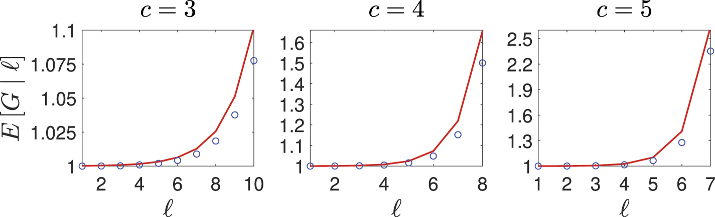
In figure 1 we present analytical results (solid lines) for the expectation value of the degeneracy $\mathbb{E}[G\vert L=\ell ]$ of shortest paths between pairs of nodes i and j as a function of the distance ℓ between them for c = 3 (left), c = 4 (center) and c = 5 (right), obtained from equation (7). The results are found to be in good agreement with the results obtained from computer simulations (circles).

Zoom In Zoom Out Reset image size

A convenient way to construct an RRG of size N and degree c (Nc must be an even number) is to prepare the N nodes such that each node is connected to c half edges or stubs [7]. At each step of the construction, one connects a pair of random stubs that belong to two different nodes i and j that are not already connected, forming an edge between them. This procedure is repeated until all the stubs are exhausted. The process may get stuck before completion whenever all the remaining stubs belong to the same node or to pairs of nodes that are already connected. In such case one needs to perform some random reconnections in order to complete the construction.

Consider an RW on an RRG that consists of N nodes of degree c ⩾ 3. Starting from a random initial node at time t = 0, at each time step t ⩾ 1 the RW hops into a random neighbor of its previous node. The probability to hop into each one of these neighbors is 1/c. For sufficiently large N the RRG consists of a single connected component, thus an RW starting from any initial node may eventually reach any other node in the network. In some of the time steps an RW may visit nodes that have not been visited before while in other time steps it may revisit nodes that have already been visited before. For example, at each time step t ⩾ 3 the RW may backtrack into the previous node with probability of 1/c. In the infinite network limit the RRG exhibits a tree structure. Therefore, in this limit the backtracking mechanism is the only way in which an RW may hop from a newly visited node to a node that has already been visited before. Such backtracking step may be followed by retroceding steps in which the RW continues to go backwards along its own path. However, in finite networks the RW may also utilize cycles to retrace its path and revisit nodes it has already visited three or more time steps earlier. In figure 2 we present a schematic illustration of some of the events that may take place along the path of an RW on an RRG. In figure 2(a) we show a path segment that includes a backtracking step, in which the RW moves back into the previous node (step no. 4). In figure 2(b) we show a path segment that includes a backtracking step (step no. 4) which is followed by a retroceding step (step no. 5). In figure 2(c) we show a path segment that includes a retracing step (step no. 6), in which the RW enters a node that was already visited five time steps earlier.

Zoom In Zoom Out Reset image size

Consider an RW on an RRG of a finite size N, starting at t = 0 from an initial node i. The time at which the RW visits a given target node j (j ≠ i) for the first time is called the first-passage time from i to j. We first consider the case in which the initial node i is random and the target node j is a random node that resides at a distance ℓ from i, where ℓ ⩾ 1. Clearly, for t < ℓ the first-passage probability satisfies P(T_FP = t|ℓ) = 0. For t ⩾ ℓ the first-passage probability satisfies P(T_FP = t|ℓ) > 0 and for any finite network

$$\begin{equation}\sum\limits _{t=\ell }^{\infty }\,P({T}_{\text{FP}}=t\vert \ell )=1.\end{equation} \tag{ 8 }$$

The probability that an RW trajectory will follow the shortest path from the initial node i to the target node j (or one of the shortest paths in case they are degenerate) is denoted by P(SPATH|ℓ). In the simplest trajectory of this type the RW moves forward along a shortest path from i to j at all time steps, such that the first-passage time is t = ℓ. However, in some of the time steps the RW may backtrack its path and possibly retrocede, resulting in a longer trajectory that still follows the shortest path. Furthermore, the RW may also step away from the shortest path and then return to the same point along the shortest path by a combination of backtracking and retroceding steps. Such trajectories are included in the SPATH scenario. More formally, for a first-passage trajectory to be an SPATH trajectory it must satisfy two conditions: (a) the subnetwork that consists of the nodes and edges along the trajectory is a tree network; (b) the distance between i and j on this subnetwork is the same as the distance ℓ_ij in the whole network. First-passage trajectories that do not satisfy one or both of these conditions are non-SPATH trajectories.

In figure 3 we present a schematic illustration of first-passage RW trajectories from the initial node i to the target node j that follow the shortest path from i to j. The simplest among these paths is an RW trajectory that goes along the shortest path without any backtracking moves or diversions (figure 3(a)). Such RW trajectories may also include backtracking and retroceding steps along the shortest path (figure 3(b)) as well as diversion segments in which the RW leaves the shortest path and then returns to the same node by retroceding its steps and then continues to follow the shortest path towards the target node j (figure 3(c)).

Zoom In Zoom Out Reset image size

The probability that an RW trajectory starting from a random initial node i will follow a shortest path (SPATH) from i to a random target node j that resides at a distance ℓ from i, and that the first-passage time will be t is denoted by P(T_FP = t, SPATH|ℓ). Clearly, for t < ℓ it satisfies P(T_FP = t, SPATH|ℓ) = 0. For t ⩾ ℓ, this probability is given by

$$\begin{equation}P({T}_{\text{FP}}=t,\mathrm{S}\mathrm{P}\mathrm{A}\mathrm{T}\mathrm{H}\vert \ell )=\begin{cases}\mathbb{E}[G\vert \ell ]B(t,\ell ){\left(\frac{1}{c}\right)}^{t}\quad \hfill & \quad t-\ell \enspace \mathrm{e}\mathrm{v}\mathrm{e}\mathrm{n}\hfill \\ 0\quad \hfill & \quad t-\ell \enspace \mathrm{o}\mathrm{d}\mathrm{d},\hfill \end{cases}\end{equation} \tag{ 9 }$$

where $\mathbb{E}[G\vert \ell ]$ is the expected number of degenerate shortest paths of length ℓ. The coefficient B(t, ℓ) is a combinatorial factor that accounts for the number of distinct RW trajectories that follow a given shortest path from i to a target node j, which resides at a distance ℓ from i, and reach j for the first time after t time steps. The term (1/c)^t accounts for the probability that an RW will follow any specific trajectory of t time steps. This is due to the fact that at each time step the probability that the RW will hop to each neighbor of the current node is 1/c. The right-hand side of equation (9) is thus a product of the total number of SPATH trajectories of t time steps by the probability that an RW will follow a given trajectory.

We now focus on a single shortest path of length ℓ between a pair of nodes i and j. The coefficients B(t, ℓ) satisfy the recursion equations

$$\begin{equation}B(t,\ell )=B(t-1,\ell -1)+(c-1)B(t-1,\ell +1),\end{equation} \tag{ 10 }$$

where the distance satisfies ℓ ⩾ 1, the first-passage time satisfies t ⩾ ℓ, and the difference t − ℓ is an even number [otherwise B(t, ℓ) = 0]. The recursion equation (10) is illustrated in figure 4, depicting a pair of nodes i and j, at a distance ℓ apart. One neighbor of i resides along the shortest path to j and is thus at a distance ℓ − 1 from j, while the other c − 1 neighbors of i are at a distance ℓ + 1 from j. Therefore, an RW trajectory starting from i and ending up at j may step at time t = 1 either into the neighbor of i that resides along the shortest path to j or into one of the other c − 1 neighbors. The boundary condition is B(ℓ, ℓ) = 1 for ℓ ⩾ 1. In the special case of ℓ = 1 and t ⩾ 3, the recursion equation is given by

$$\begin{equation}B(t,1)=(c-1)B(t-1,2).\end{equation} \tag{ 11 }$$

Actually, the B(t, ℓ) coefficients are also defined for ℓ = 0. In this case, they provide the number of RW trajectories that return to the initial node for the first time at time t, and are thus important in the analysis of the FR problem, recently studied in reference [22].

Zoom In Zoom Out Reset image size

In appendix A we present a solution of the recursion relations given by equation (10) for ℓ ⩾ 1 and t ⩾ ℓ with the boundary conditions specified above. It is found that for any distance ℓ ⩾ 1 between the initial node i and the target node j and for any time t ⩾ ℓ the number of distinct RW trajectories that follow a given shortest path from i to j and for which the first-passage time is t, is given by

$$\begin{equation}B(t,\ell )=\begin{cases}\frac{\ell }{t}\left(\genfrac{}{}{0.0pt}{}{t}{\frac{t+\ell }{2}}\right){(c-1)}^{\frac{t-\ell }{2}}\quad \hfill & \quad t-\ell \enspace \mathrm{e}\mathrm{v}\mathrm{e}\mathrm{n}\hfill \\ 0\quad \hfill & \quad t-\ell \enspace \mathrm{o}\mathrm{d}\mathrm{d},\hfill \end{cases}\end{equation} \tag{ 12 }$$

where $\left(\genfrac{}{}{0.0pt}{}{n}{m}\right)$ is the binomial coefficient. The coefficient B(t, ℓ) captures the contribution of a single shortest path to the distribution of first passage times via the SPATH scenario.

In order to proceed one needs to account for the contributions of all the degenerate shortest paths between the initial node and the target node. The probability that an RW starting from a random initial node i will reach a random target node j that resides at a distance ℓ from i for the first time via the SPATH scenario is given by

$$\begin{equation}P(\mathrm{S}\mathrm{P}\mathrm{A}\mathrm{T}\mathrm{H}\vert \ell )=\sum\limits _{t=\ell }^{\infty }\,P({T}_{\text{FP}}=t,\mathrm{S}\mathrm{P}\mathrm{A}\mathrm{T}\mathrm{H}\vert \ell ).\end{equation} \tag{ 13 }$$

Inserting P(T_FP = t, SPATH|ℓ) from equation (9) [with B(t, ℓ) from equation (12)] into equation (13) and carrying out the summation, we obtain

$$\begin{equation}P(\mathrm{S}\mathrm{P}\mathrm{A}\mathrm{T}\mathrm{H}\vert \ell )={\left(\frac{1}{c-1}\right)}^{\ell }\mathbb{E}[G\vert \ell ].\end{equation} \tag{ 14 }$$

The first term on the right-hand side of equation (14) accounts for the contribution of a single shortest path while the second term accounts for the expected number of such paths. Inserting the approximated result for the degeneracy $\mathbb{E}[G\vert \ell ]$, given by equation (7), into equation (14), we obtain

$$\begin{equation}P(\mathrm{S}\mathrm{P}\mathrm{A}\mathrm{T}\mathrm{H}\vert \ell )\simeq {\left(\frac{1}{c-1}\right)}^{\ell }+\frac{1}{N}.\end{equation} \tag{ 15 }$$

The first term in equation (15) accounts for the contribution of the single shortest path which is guaranteed to exist, given that the distance between the initial node i and the target node j is equal to ℓ. The second term accounts for the expected contribution of degenerate shortest paths of length ℓ.

The complementary probability is given by

$$\begin{equation}P({\neg}\mathrm{S}\mathrm{P}\mathrm{A}\mathrm{T}\mathrm{H}\vert \ell )\simeq 1-{\left(\frac{1}{c-1}\right)}^{\ell }-\frac{1}{N}.\end{equation} \tag{ 16 }$$

In figure 5 we present analytical results (solid lines) for the probability P(SPATH|ℓ) that the first-passage of an RW from a random initial node i to a random target node j which is at a distance ℓ from i, will take place via the SPATH scenario, as a function of the distance ℓ. The results are shown for RRGs of size N = 1000 and c = 3 (left), c = 4 (center) and c = 10 (right). The analytical results, obtained from equation (15) are found to be in good agreement with the results obtained from computer simulations (circles).

Zoom In Zoom Out Reset image size

The distribution of first-passage times via SPATH trajectories, from a random node i to a random node j that resides at a distance ℓ from i, is given by

$$\begin{equation}P({T}_{\text{FP}}=t\vert \ell ,\mathrm{S}\mathrm{P}\mathrm{A}\mathrm{T}\mathrm{H})=\frac{P({T}_{\text{FP}}=t,\mathrm{S}\mathrm{P}\mathrm{A}\mathrm{T}\mathrm{H}\vert \ell )}{P(\mathrm{S}\mathrm{P}\mathrm{A}\mathrm{T}\mathrm{H}\vert \ell )}.\end{equation} \tag{ 17 }$$

Plugging in P(T_FP = t, SPATH|ℓ) from equation (9) and P(SPATH|ℓ) from equation (14) into equation (17), it is found that P(T_FP = t|ℓ, SPATH) = 0 for t < ℓ, while for t ⩾ ℓ it is given by

$$\begin{equation}P({T}_{\text{FP}}=t\vert \ell ,\mathrm{S}\mathrm{P}\mathrm{A}\mathrm{T}\mathrm{H})=\begin{cases}\frac{\ell }{t}\left(\genfrac{}{}{0.0pt}{}{t}{\frac{t+\ell }{2}}\right){\left(1-\frac{1}{c}\right)}^{\frac{t+\ell }{2}}{\left(\frac{1}{c}\right)}^{\frac{t-\ell }{2}}\quad \hfill & \quad t-\ell \enspace \mathrm{e}\mathrm{v}\mathrm{e}\mathrm{n}\hfill \\ 0\quad \hfill & \quad t-\ell \enspace \mathrm{o}\mathrm{d}\mathrm{d}.\hfill \end{cases}\end{equation} \tag{ 18 }$$

The corresponding tail distribution is given by

$$\begin{equation}P({T}_{\text{FP}} > t\vert \ell ,\mathrm{S}\mathrm{P}\mathrm{A}\mathrm{T}\mathrm{H})=\sum\limits _{{t}^{\prime }=t+1}^{\infty }\,P({T}_{\text{FP}}={t}^{\prime }\vert \ell ,\mathrm{S}\mathrm{P}\mathrm{A}\mathrm{T}\mathrm{H}).\end{equation} \tag{ 19 }$$

In figure 6 we present analytical results (solid line) for the tail distribution P(T_FP > t|ℓ, SPATH) of first-passage times for RW trajectories that follow the shortest path between pairs of nodes which are at a distance ℓ from each other, for ℓ = 1 (left), ℓ = 2 (center) and ℓ = 3 (right). The results are shown for RRGs of size N = 1000 and degree c = 3. The analytical results, obtained from equation (19) are in very good agreement with the results obtained from computer simulations (circles).

Zoom In Zoom Out Reset image size

The generating function of the distribution P(T_FP = t|ℓ, SPATH) is given by

$$\begin{equation}{V}_{\ell }(x)=\sum\limits _{t=1}^{\infty }\,{x}^{t}P({T}_{\text{FP}}=t\vert \ell ,\mathrm{S}\mathrm{P}\mathrm{A}\mathrm{T}\mathrm{H}).\end{equation} \tag{ 20 }$$

Such generating functions were studied extensively in the context of RWs on regular lattices [13]. Inserting P(T_FP = t|ℓ, SPATH) from equation (18) into equation (20) and carrying out the summation, we obtain

$$\begin{equation}{V}_{\ell }(x)={\left(1-\frac{1}{c}\right)}^{\ell }{x}^{\ell }\,{}_{2}F_{1}\left[\left.\begin{matrix}\hfill \frac{\ell }{2},\frac{\ell +1}{2}\hfill \\ \hfill \ell +1\hfill \end{matrix}\right\vert \frac{4(c-1)}{{c}^{2}}{x}^{2}\right],\end{equation} \tag{ 21 }$$

where ${}_{2}F_{1}\left[\left.\begin{matrix}\hfill a,b\hfill \\ \hfill c\hfill \end{matrix}\right\vert z\right]$ is the hypergeometric function [33]. Applying identity (A.16) from appendix A on the hypergeometric function on the right-hand side of equation (21), it can be simplified to

$$\begin{equation}{V}_{\ell }(x)={\left[\frac{c-\sqrt{{c}^{2}-4(c-1){x}^{2}}}{2x}\right]}^{\ell }.\end{equation} \tag{ 22 }$$

The r'th moment of P(T_FP = t|ℓ, SPATH) is given by

$$\begin{equation}\mathbb{E}[{T}_{\text{FP}}^{r}\vert \ell ,\mathrm{S}\mathrm{P}\mathrm{A}\mathrm{T}\mathrm{H}]=\sum\limits _{t=1}^{\infty }\,{t}^{r}P({T}_{\text{FP}}=t\vert \ell ,\mathrm{S}\mathrm{P}\mathrm{A}\mathrm{T}\mathrm{H}).\end{equation} \tag{ 23 }$$

Inserting r = 1 in equation (23) we obtain the mean first-passage time $\mathbb{E}[{T}_{\text{FP}}\vert \ell ,\mathrm{S}\mathrm{P}\mathrm{A}\mathrm{T}\mathrm{H}]$. It can also be obtained directly from the generating function V_ℓ (x) by

$$\begin{equation}\mathbb{E}[{T}_{\text{FP}}\vert \ell ,\mathrm{S}\mathrm{P}\mathrm{A}\mathrm{T}\mathrm{H}]={\left.\frac{\mathrm{d}{V}_{\ell }(x)}{\mathrm{d}x}\right\vert }_{x=1},\end{equation} \tag{ 24 }$$

which yields

$$\begin{equation}\mathbb{E}[{T}_{\text{FP}}\vert \ell ,\mathrm{S}\mathrm{P}\mathrm{A}\mathrm{T}\mathrm{H}]=\frac{c}{c-2}\ell .\end{equation} \tag{ 25 }$$

The second factorial moment is given by

$$\begin{equation}\mathbb{E}[{T}_{\text{FP}}({T}_{\text{FP}}-1)\vert \ell ,\mathrm{S}\mathrm{P}\mathrm{A}\mathrm{T}\mathrm{H}]={\left.\frac{{\mathrm{d}}^{2}{V}_{\ell }(x)}{\mathrm{d}{x}^{2}}\right\vert }_{x=1},\end{equation} \tag{ 26 }$$

which yields

$$\begin{equation}\mathbb{E}[{T}_{\text{FP}}({T}_{\text{FP}}-1)\vert \ell ,\mathrm{S}\mathrm{P}\mathrm{A}\mathrm{T}\mathrm{H}]=\frac{{c}^{2}{\ell }^{2}}{{(c-2)}^{2}}-\frac{{c}^{2}-8c+8}{{(c-2)}^{2}}c\ell .\end{equation} \tag{ 27 }$$

Combining the results for the first moment and the second factorial moment, we obtain

$$\begin{equation}\mathbb{E}[{T}_{\text{FP}}^{2}\vert \ell ,\mathrm{S}\mathrm{P}\mathrm{A}\mathrm{T}\mathrm{H}]=\frac{4c(c-1)}{{(c-2)}^{3}}\ell +{\left(\frac{c}{c-2}\right)}^{2}{\ell }^{2}.\end{equation} \tag{ 28 }$$

Using the results presented above for the first and second moments we obtain the variance, which is given by

$$\begin{equation}\mathrm{Var}[{T}_{\text{FP}}\vert \ell ,\mathrm{S}\mathrm{P}\mathrm{A}\mathrm{T}\mathrm{H}]=\frac{4c(c-1)}{{(c-2)}^{3}}\ell .\end{equation} \tag{ 29 }$$

The probability that the first-passage trajectory of an RW from a random initial node i to a random target node j in an RRG of a finite size N will follow the shortest path from i to j is given by

$$\begin{equation}P(\mathrm{S}\mathrm{P}\mathrm{A}\mathrm{T}\mathrm{H})=\sum\limits _{\ell =1}^{N-1}\,P(\mathrm{S}\mathrm{P}\mathrm{A}\mathrm{T}\mathrm{H}\vert \ell )P(L=\ell ),\end{equation} \tag{ 30 }$$

where P(SPATH|ℓ) is given by equation (14) and P(L = ℓ) is given by equations (1)–(4). Using equation (4), we obtain

$$\begin{equation}P(\mathrm{S}\mathrm{P}\mathrm{A}\mathrm{T}\mathrm{H})=\sum\limits _{\ell =1}^{N-1}\,P(\mathrm{S}\mathrm{P}\mathrm{A}\mathrm{T}\mathrm{H}\vert \ell )\left[P(L > \ell -1)-P(L > \ell )\right].\end{equation} \tag{ 31 }$$

Rearranging the summation indices, we obtain

$$\begin{equation}P(\mathrm{S}\mathrm{P}\mathrm{A}\mathrm{T}\mathrm{H})=P(\mathrm{S}\mathrm{P}\mathrm{A}\mathrm{T}\mathrm{H}\vert 1)+\sum\limits _{\ell =1}^{N-2}\left[P(\mathrm{S}\mathrm{P}\mathrm{A}\mathrm{T}\mathrm{H}\vert \ell +1)-P(\mathrm{S}\mathrm{P}\mathrm{A}\mathrm{T}\mathrm{H}\vert \ell )\right]P(L > \ell ).\end{equation} \tag{ 32 }$$

The transformation from equation (30) to equation (32) essentially amounts to a summation by parts. Inserting P(SPATH|ℓ) from equation (14) into equation (32) and rearranging terms, we obtain

$$\begin{equation}P(\mathrm{S}\mathrm{P}\mathrm{A}\mathrm{T}\mathrm{H})\simeq 1+\frac{1}{N}-\frac{c-2}{c-1}\sum\limits _{\ell =0}^{N-1}{\left(\frac{1}{c-1}\right)}^{\ell }P(L > \ell ),\end{equation} \tag{ 33 }$$

where we use the fact that P(L > 0) = 1. Clearly, the upper limit of the summation in equation (33) can be replaced by ∞ with negligible effect on the result. Using the definition of b from equation (3), we rewrite equation (33) in the form

$$\begin{equation}P(\mathrm{S}\mathrm{P}\mathrm{A}\mathrm{T}\mathrm{H})\simeq 1+\frac{1}{N}-\frac{c-2}{c-1}\sum\limits _{\ell =0}^{\infty }{\mathrm{e}}^{-b\ell }P(L > \ell ).\end{equation} \tag{ 34 }$$

It can also be written in the form

$$\begin{equation}P(\mathrm{S}\mathrm{P}\mathrm{A}\mathrm{T}\mathrm{H})\simeq 1+\frac{1}{N}-\frac{c-2}{c-1}{M}_{0}\end{equation} \tag{ 35 }$$

where

$$\begin{equation}{M}_{0}=\mathcal{L}[P(L > \ell )](s=b)=\sum\limits _{\ell =0}^{\infty }{\mathrm{e}}^{-b\ell }P(L > \ell )\end{equation} \tag{ 36 }$$

and $\mathcal{L}[P(L > \ell )](s)$ is the discrete Laplace transform (or the unilateral Z-transform) of the tail distribution P(L > ℓ), evaluated at s = b. An explicit expression for M₀ is given by equation (B.8). It is based on a recent calculation of the discrete Laplace transform $\mathcal{L}[P(L > \ell )](s)$ [32]. In the large network limit it can be reduced to equation (B.9).

Equations (33)–(36) provide an interesting relation between the geometric properties of the network, captured by P(L > ℓ), and the probability P(SPATH) which is a dynamical property of the RW trajectories. It exemplifies the potential use of the DSPL in the analysis of dynamical processes on networks. Inserting M₀ from equations (B.9) into (35) and rearranging terms, we obtain

$$\begin{equation}P(\mathrm{S}\mathrm{P}\mathrm{A}\mathrm{T}\mathrm{H})\simeq \left(\frac{c}{c-1}\right)\frac{1}{N}\left[\frac{\ln \left(\frac{c-2}{c}N\right)-\gamma +1}{\ln (c-1)}+\frac{{c}^{2}-6c+4}{2c(c-2)}\right]+\mathcal{O}\left(\frac{1}{{N}^{2}}\right),\end{equation} \tag{ 37 }$$

where γ is the Euler–Mascheroni constant [33]. Using the result for the mean distance ⟨L⟩, presented in [32], equation (37) can be written in the form

$$\begin{equation}P(\mathrm{S}\mathrm{P}\mathrm{A}\mathrm{T}\mathrm{H})\simeq \left(\frac{c}{c-1}\right)\frac{1}{N}\left[\langle L\rangle +\frac{1}{\ln (c-1)}-2\frac{c-1}{c(c-2)}\right]+\mathcal{O}\left(\frac{1}{{N}^{2}}\right).\end{equation} \tag{ 38 }$$

In the limit of large and dense networks, equation (38) can be simplified to

$$\begin{equation}P(\mathrm{S}\mathrm{P}\mathrm{A}\mathrm{T}\mathrm{H})\simeq \left(\frac{c}{c-1}\right)\frac{\langle L\rangle }{N}+\mathcal{O}\left[\frac{1}{N\ln (c-1)}\right].\end{equation} \tag{ 39 }$$

In the infinite network limit one expects the probability P(SPATH) to vanish. This is due to the fact that as N is increased (keeping c constant) the typical distance between pairs of random nodes increases. Thus the probability that an RW starting from a random initial node will follow the shortest path to a random target node decreases as N is increased.

In figure 7 we present analytical results (solid line) for the probability P(SPATH) that the first-passage of an RW from a random initial node i to a random target node j will occur via the SPATH scenario on RRGs of size N = 1000 as a function of the degree c. The analytical results are obtained from equation (35), where M₀ is given by equation (B.8). They are found to be in very good agreement with the results obtained from computer simulations. The simulations are performed on an ensemble of RRGs that are constructed using the procedure presented in section 2. For each instance of a first-passage RW trajectory we select a random initial node i and a random target node j. The trajectory of an RW that starts from node i is recorded until it visits node j for the first time. In order to qualify as an SPATH trajectory it should pass two tests. First, it should not include any cycles. This means that the subgraph consisting of the nodes that the RW visited and the edges it used along the way from i to j must be a tree. Second, the distance between i and j on this subgraph must be equal to the distance between i and j on the underlying RRG. The fraction of first-passage RW trajectories that meet these two criteria is used to estimate P(SPATH).

Zoom In Zoom Out Reset image size

The distribution of first-passage times from a random initial node i to a random target node j, under the condition that the RW follows the shortest path from i to j, is given by

$$\begin{equation}P({T}_{\text{FP}}=t\vert \mathrm{S}\mathrm{P}\mathrm{A}\mathrm{T}\mathrm{H})=\sum\limits _{\ell =1}^{t}\,P({T}_{\text{FP}}=t\vert \ell ,\mathrm{S}\mathrm{P}\mathrm{A}\mathrm{T}\mathrm{H})P(L=\ell \vert \mathrm{S}\mathrm{P}\mathrm{A}\mathrm{T}\mathrm{H}),\end{equation} \tag{ 40 }$$

where

$$\begin{equation}P(L=\ell \vert \mathrm{S}\mathrm{P}\mathrm{A}\mathrm{T}\mathrm{H})=\frac{P(\mathrm{S}\mathrm{P}\mathrm{A}\mathrm{T}\mathrm{H}\vert \ell )P(L=\ell )}{P(\mathrm{S}\mathrm{P}\mathrm{A}\mathrm{T}\mathrm{H})}.\end{equation} \tag{ 41 }$$

The probability P(T_FP = t|ℓ, SPATH) makes a non-vanishing contribution to the sum only for even (and non-negative) values of t − ℓ. Therefore, in equation (40) we need to distinguish between even and odd values of t. In case that t is even, the sum on the right-hand side is over even values of ℓ, while if t is odd the sum is over odd values of ℓ. Inserting P(T_FP = t|ℓ, SPATH) from equation (18) into equation (40), we find that for even values of the time t

$$\begin{align}\hfill P({T}_{\text{FP}}=t\vert \mathrm{S}\mathrm{P}\mathrm{A}\mathrm{T}\mathrm{H})& \simeq \frac{{(c-1)}^{\frac{t}{2}}}{t{c}^{t}P(\mathrm{S}\mathrm{P}\mathrm{A}\mathrm{T}\mathrm{H})}\hfill \\ \hfill & \quad \times \sum\limits _{k=1}^{\frac{t}{2}}\frac{2k}{{(c-1)}^{k}}\left(\genfrac{}{}{0.0pt}{}{t}{\frac{t}{2}+k}\right)\left[1+\frac{{(c-1)}^{2k}}{N}\right]P(L=2k),\hfill \end{align} \tag{ 42 }$$

while for odd values of t

$$\begin{align}\hfill P({T}_{\text{FP}}=t\vert \mathrm{S}\mathrm{P}\mathrm{A}\mathrm{T}\mathrm{H})\simeq \frac{{(c-1)}^{\frac{t+1}{2}}}{t{c}^{t}P(\mathrm{S}\mathrm{P}\mathrm{A}\mathrm{T}\mathrm{H})}\\ \hfill & \times \sum\limits _{k=1}^{\frac{t+1}{2}}\frac{2k-1}{{(c-1)}^{k}}\left(\genfrac{}{}{0.0pt}{}{t}{\frac{t-1}{2}+k}\right)\left[1+\frac{{(c-1)}^{2k-1}}{N}\right]P(L=2k-1).\hfill \end{align} \tag{ 43 }$$

The tail distribution of first-passage times in the SPATH scenario is given by

$$\begin{equation}P({T}_{\text{FP}} > t\vert \mathrm{S}\mathrm{P}\mathrm{A}\mathrm{T}\mathrm{H})=\sum\limits _{{t}^{\prime }=t+1}^{\infty }\,P({T}_{\text{FP}}={t}^{\prime }\vert \mathrm{S}\mathrm{P}\mathrm{A}\mathrm{T}\mathrm{H}).\end{equation} \tag{ 44 }$$

In figure 8 we present analytical results for the tail distribution P(T_FP > t|SPATH) of first-passage times (solid lines) for RW trajectories that follow the shortest path from a random initial node i to a random target node j on an RRG of size N = 1000 and degrees c = 3, c = 4 and c = 10. The analytical results, obtained from equation (44) are in very good agreement with the results obtained from computer simulations (circles).

Zoom In Zoom Out Reset image size

The first and second moments of the distribution of first-passage times between a random initial node i and a random target node j, under the condition that the RW follows the shortest path between i and j are given by

$$\begin{equation}\mathbb{E}[{T}_{\text{FP}}^{r}\vert \mathrm{S}\mathrm{P}\mathrm{A}\mathrm{T}\mathrm{H}]=\sum\limits _{\ell =1}^{N-1}\,\mathbb{E}[{T}_{\text{FP}}^{r}\vert \ell ,\mathrm{S}\mathrm{P}\mathrm{A}\mathrm{T}\mathrm{H}]P(L=\ell \vert \mathrm{S}\mathrm{P}\mathrm{A}\mathrm{T}\mathrm{H}),\end{equation} \tag{ 45 }$$

where r = 1 and 2, respectively. Inserting the first moment $\mathbb{E}[{T}_{\text{FP}}\vert \ell ,\mathrm{S}\mathrm{P}\mathrm{A}\mathrm{T}\mathrm{H}]$ from equation (25) into (45) and carrying out the summation, we obtain

$$\begin{equation}\mathbb{E}[{T}_{\text{FP}}\vert \mathrm{S}\mathrm{P}\mathrm{A}\mathrm{T}\mathrm{H}]\simeq \frac{1}{P(\mathrm{S}\mathrm{P}\mathrm{A}\mathrm{T}\mathrm{H})}\left(\frac{c}{c-2}\right)\sum\limits _{\ell =1}^{N-1}\,\ell \left[{\left(\frac{1}{c-1}\right)}^{\ell }+\frac{1}{N}\right]P(L=\ell ).\end{equation} \tag{ 46 }$$

Using summation by parts and collecting terms, we obtain

$$\begin{equation}\mathbb{E}[{T}_{\text{FP}}\vert \mathrm{S}\mathrm{P}\mathrm{A}\mathrm{T}\mathrm{H}]\simeq \frac{1}{P(\mathrm{S}\mathrm{P}\mathrm{A}\mathrm{T}\mathrm{H})}\left(\frac{c}{c-2}\right)\left[\frac{\langle L\rangle }{N}+\frac{1}{c-1}\sum\limits _{\ell =0}^{N-1}\frac{1-(c-2)\ell }{{(c-1)}^{\ell }}P(L > \ell )\right].\end{equation} \tag{ 47 }$$

Using the results presented in appendix B for the sums M₀ and M₁, we obtain

$$\begin{equation}\mathbb{E}[{T}_{\text{FP}}\vert \mathrm{S}\mathrm{P}\mathrm{A}\mathrm{T}\mathrm{H}]\simeq \frac{1}{P(\mathrm{S}\mathrm{P}\mathrm{A}\mathrm{T}\mathrm{H})}\left(\frac{c}{c-2}\right)\left[\frac{\langle L\rangle }{N}+\frac{{M}_{0}-(c-2){M}_{1}}{c-1}\right],\end{equation} \tag{ 48 }$$

where M₀ is given by equation (B.8), M₁ is given by equation (B.10) and ⟨L⟩ is the mean distance. In the large network limit, one can express M₀ by equation (B.9), M₁ by equation (B.12) and P(SPATH) by equation (38). This yields

$$\begin{equation}\mathbb{E}[{T}_{\text{FP}}\vert \mathrm{S}\mathrm{P}\mathrm{A}\mathrm{T}\mathrm{H}]\simeq \frac{1}{2}\left(\frac{c}{c-2}\right)\left[\langle L\rangle +1-4\frac{c-1}{c(c-2)}+\frac{2}{\ln (c-1)}\right]+\mathcal{O}\left(\frac{1}{\ln \,N}\right).\end{equation} \tag{ 49 }$$

The variance can be calculated by applying a similar approach to equation (29). It yields

$$\begin{equation}\mathrm{Var}[{T}_{\text{FP}}\vert \mathrm{S}\mathrm{P}\mathrm{A}\mathrm{T}\mathrm{H}]\simeq \frac{1}{P(\mathrm{S}\mathrm{P}\mathrm{A}\mathrm{T}\mathrm{H})}\frac{4c(c-1)}{{(c-2)}^{3}}\left[\frac{\langle L\rangle }{N}+\frac{{M}_{0}-(c-2){M}_{1}}{c-1}\right].\end{equation} \tag{ 50 }$$

Comparing equations (48) and (50) it is found that

$$\begin{equation}\mathrm{Var}[{T}_{\text{FP}}\vert \mathrm{S}\mathrm{P}\mathrm{A}\mathrm{T}\mathrm{H}]\simeq 4\frac{c-1}{{(c-2)}^{2}}\mathbb{E}[{T}_{\text{FP}}\vert \mathrm{S}\mathrm{P}\mathrm{A}\mathrm{T}\mathrm{H}].\end{equation} \tag{ 51 }$$

This implies that the distribution P(T_FP|SPATH) becomes narrower as c is increased.

In this section we derive a closed form expression for the distribution P(T_FP > t|¬SPATH) of first-passage times between a random initial node i and a random target node j, under the condition that the first-passage trajectory does not follow the shortest path from i to j. In case that the distance ℓ between i and j is known, the distribution of first-passage times, conditioned on ℓ, is denoted by P(T_FP > t|ℓ, ¬SPATH). Since an RW trajectory from i to j that does not follow the shortest path must be longer than ℓ, we conclude that P(T_FP > t|ℓ, ¬SPATH) = 1 for t ⩽ ℓ.

Starting from a random initial node i the RW visits, on average, ⟨S⟩_t distinct nodes up to time t. In case that the distance between i and j is ℓ, the earliest time at which the RW may visit the target node via a trajectory that does not follow the shortest path is t = ℓ + 1. Therefore, the tail distribution of first-passage times, conditioned on the distance ℓ, satisfies

$$\begin{equation}P({T}_{\text{FP}} > t\vert \ell ,{\neg}\mathrm{S}\mathrm{P}\mathrm{A}\mathrm{T}\mathrm{H})=1-\frac{{\langle S\rangle }_{t-\ell }}{N},\end{equation} \tag{ 52 }$$

where [22, 34]

$$\begin{equation}{\langle S\rangle }_{t}=N\left[1-{\mathrm{e}}^{-\left(\frac{c-2}{c-1}\right)\frac{t}{N}}\right].\end{equation} \tag{ 53 }$$

Inserting ⟨S⟩_t from equation (53) into equation (52), we obtain

$$\begin{equation}P({T}_{\text{FP}} > t\vert \ell ,{\neg}\mathrm{S}\mathrm{P}\mathrm{A}\mathrm{T}\mathrm{H})=\begin{cases}1\quad \hfill & \quad t\leqslant \ell \hfill \\ \mathrm{exp}\left[-\left(\frac{c-2}{c-1}\right)\frac{t-\ell }{N}\right]\quad \hfill & \quad t > \ell .\hfill \end{cases}\end{equation} \tag{ 54 }$$

The tail distribution of first-passage times is given by

$$\begin{equation}P({T}_{\text{FP}} > t\vert {\neg}\mathrm{S}\mathrm{P}\mathrm{A}\mathrm{T}\mathrm{H})=\sum\limits _{\ell =1}^{\infty }\,P({T}_{\text{FP}} > t\vert \ell ,{\neg}\mathrm{S}\mathrm{P}\mathrm{A}\mathrm{T}\mathrm{H})P(L=\ell \vert {\neg}\mathrm{S}\mathrm{P}\mathrm{A}\mathrm{T}\mathrm{H}),\end{equation} \tag{ 55 }$$

where

$$\begin{equation}P(L=\ell \vert {\neg}\mathrm{S}\mathrm{P}\mathrm{A}\mathrm{T}\mathrm{H})=\frac{P({\neg}\mathrm{S}\mathrm{P}\mathrm{A}\mathrm{T}\mathrm{H}\vert \ell )P(L=\ell )}{P({\neg}\mathrm{S}\mathrm{P}\mathrm{A}\mathrm{T}\mathrm{H})}.\end{equation} \tag{ 56 }$$

In equation (56) the probability P(¬SPATH|ℓ) is given by equation (16) and the probability P(¬SPATH) = 1 − P(SPATH), where P(SPATH) is given by equation (35). Inserting P(T_FP > t|ℓ, ¬SPATH) from equation (54) into equation (55), we obtain

$$\begin{align}\hfill P({T}_{\text{FP}} > t\vert {\neg}\mathrm{S}\mathrm{P}\mathrm{A}\mathrm{T}\mathrm{H})& =\sum\limits _{\ell =t+1}^{\infty }\,P(L=\ell \vert {\neg}\mathrm{S}\mathrm{P}\mathrm{A}\mathrm{T}\mathrm{H})\hfill \\ \hfill & \quad +\mathrm{exp}\left[-\left(\frac{c-2}{c-1}\right)\frac{t}{N}\right]\sum\limits _{\ell =1}^{t}\mathrm{exp}\left[\left(\frac{c-2}{c-1}\right)\frac{\ell }{N}\right]\hfill \\ \hfill & \quad \times P(L=\ell \vert {\neg}\mathrm{S}\mathrm{P}\mathrm{A}\mathrm{T}\mathrm{H}).\hfill \end{align} \tag{ 57 }$$

Since the diameter of an RRG scales logarithmically with the network size [35], in the large network limit and for t ≫ ln N equation (57) can be simplified to the form

$$\begin{equation}P({T}_{\text{FP}} > t\vert {\neg}\mathrm{S}\mathrm{P}\mathrm{A}\mathrm{T}\mathrm{H})=\mathrm{exp}\left[-\left(\frac{c-2}{c-1}\right)\frac{t}{N}\right].\end{equation} \tag{ 58 }$$

The conditional probability mass function of first-passage times for trajectories that do not follow the shortest path is given by

$$\begin{align}\hfill P({T}_{\text{FP}}=t\vert {\neg}\mathrm{S}\mathrm{P}\mathrm{A}\mathrm{T}\mathrm{H})& =P({T}_{\text{FP}} > t-1\vert {\neg}\mathrm{S}\mathrm{P}\mathrm{A}\mathrm{T}\mathrm{H})\,-P({T}_{\text{FP}} > t\vert {\neg}\mathrm{S}\mathrm{P}\mathrm{A}\mathrm{T}\mathrm{H}).\hfill \end{align} \tag{ 59 }$$

Inserting P(T_FP > t|¬SPATH) from equation (58) into equation (59) we obtain

$$\begin{equation}P({T}_{\text{FP}}=t\vert {\neg}\mathrm{S}\mathrm{P}\mathrm{A}\mathrm{T}\mathrm{H})=\left\{\mathrm{exp}\left[\left(\frac{c-2}{c-1}\right)\frac{1}{N}\right]-1\right\}\mathrm{exp}\left[-\left(\frac{c-2}{c-1}\right)\frac{t}{N}\right].\end{equation} \tag{ 60 }$$

In the large network limit, where N ≫ 1, equation (60) can be approximated by

$$\begin{equation}P({T}_{\text{FP}}=t\vert {\neg}\mathrm{S}\mathrm{P}\mathrm{A}\mathrm{T}\mathrm{H})=\left(\frac{c-2}{c-1}\right)\frac{1}{N}\mathrm{exp}\left[-\left(\frac{c-2}{c-1}\right)\frac{t}{N}\right].\end{equation} \tag{ 61 }$$

The moments $\mathbb{E}[{T}_{\text{FP}}^{r}\vert {\neg}\mathrm{S}\mathrm{P}\mathrm{A}\mathrm{T}\mathrm{H}]$, r = 1, 2, ..., can be obtained from the tail-sum formula [36]

$$\begin{equation}\mathbb{E}[{T}_{\text{FP}}^{r}\vert {\neg}\mathrm{S}\mathrm{P}\mathrm{A}\mathrm{T}\mathrm{H}]=\sum\limits _{t=0}^{\infty }[{(t+1)}^{r}-{t}^{r}]P({T}_{\text{FP}} > t\vert {\neg}\mathrm{S}\mathrm{P}\mathrm{A}\mathrm{T}\mathrm{H}).\end{equation} \tag{ 62 }$$

In particular, the mean first-passage time $\mathbb{E}[{T}_{\text{FP}}\vert {\neg}\mathrm{S}\mathrm{P}\mathrm{A}\mathrm{T}\mathrm{H}]$ can be obtained by inserting r = 1 in equation (62), which yields

$$\begin{equation}\mathbb{E}[{T}_{\text{FP}}\vert {\neg}\mathrm{S}\mathrm{P}\mathrm{A}\mathrm{T}\mathrm{H}]=\sum\limits _{t=0}^{\infty }\,P({T}_{\text{FP}} > t\vert {\neg}\mathrm{S}\mathrm{P}\mathrm{A}\mathrm{T}\mathrm{H}).\end{equation} \tag{ 63 }$$

Similarly, inserting r = 2 in equation (62) we obtain the second moment $\mathbb{E}[{T}_{\text{FP}}^{2}\vert {\neg}\mathrm{S}\mathrm{P}\mathrm{A}\mathrm{T}\mathrm{H}]$ of the distribution of first-passage times, which is given by

$$\begin{equation}\mathbb{E}[{T}_{\text{FP}}^{2}\vert {\neg}\mathrm{S}\mathrm{P}\mathrm{A}\mathrm{T}\mathrm{H}]=\sum\limits _{t=0}^{\infty }(2t+1)P({T}_{\text{FP}} > t\vert {\neg}\mathrm{S}\mathrm{P}\mathrm{A}\mathrm{T}\mathrm{H}).\end{equation} \tag{ 64 }$$

Inserting the tail distribution of equation (58) into equation (63) we obtain the mean first-passage time, which is given by

$$\begin{equation}\mathbb{E}[{T}_{\text{FP}}\vert {\neg}\mathrm{S}\mathrm{P}\mathrm{A}\mathrm{T}\mathrm{H}]=\frac{1}{1-\mathrm{exp}\left[-\left(\frac{c-2}{c-1}\right)\frac{1}{N}\right]}.\end{equation} \tag{ 65 }$$

In the large network limit, where N ≫ 1, equation (65) can be approximated by

$$\begin{equation}\mathbb{E}[{T}_{\text{FP}}\vert {\neg}\mathrm{S}\mathrm{P}\mathrm{A}\mathrm{T}\mathrm{H}]\simeq \frac{c-1}{c-2}N,\end{equation} \tag{ 66 }$$

where c ⩾ 3. The result of equation (66) was obtained in [37] using different considerations. Interestingly, in the dense network limit of c ≫ 1 it is found that ⟨T_FP⟩ ≃ N, while in the dilute network limit of c = 3, ⟨T_FP⟩ ≃ 2N. This reflects the larger fraction of backtracking steps in RRGs of low degree.

Inserting the tail distribution of equation (58) into equation (64) we obtain the second moment

$$\begin{equation}\mathbb{E}[{T}_{\text{FP}}^{2}\vert {\neg}\mathrm{S}\mathrm{P}\mathrm{A}\mathrm{T}\mathrm{H}]=\frac{1+\mathrm{exp}\left[-\left(\frac{c-2}{c-1}\right)\frac{1}{N}\right]}{{\left\{1-\mathrm{exp}\left[-\left(\frac{c-2}{c-1}\right)\frac{1}{N}\right]\right\}}^{2}}.\end{equation} \tag{ 67 }$$

Combining the results for the first and second moments, we obtain the variance, which is given by

$$\begin{equation}\mathrm{Var}[{T}_{\text{FP}}\vert {\neg}\mathrm{S}\mathrm{P}\mathrm{A}\mathrm{T}\mathrm{H}]=\frac{\mathrm{exp}\left[-\frac{c-2}{(c-1)N}\right]}{{\left\{1-\mathrm{exp}\left[-\frac{c-2}{(c-1)N}\right]\right\}}^{2}}.\end{equation} \tag{ 68 }$$

For any value of the distance ℓ between the initial node i and the target node j, the conditional distribution of first-passage times can be written in the form

$$\begin{align}\hfill P({T}_{\text{FP}}=t\vert \ell )& =P({T}_{\text{FP}}=t\vert \ell ,\mathrm{S}\mathrm{P}\mathrm{A}\mathrm{T}\mathrm{H})P(\mathrm{S}\mathrm{P}\mathrm{A}\mathrm{T}\mathrm{H}\vert \ell )\hfill \\ \hfill & \quad +P({T}_{\text{FP}}=t\vert \ell ,{\neg}\mathrm{S}\mathrm{P}\mathrm{A}\mathrm{T}\mathrm{H})P({\neg}\mathrm{S}\mathrm{P}\mathrm{A}\mathrm{T}\mathrm{H}\vert \ell ),\hfill \end{align} \tag{ 69 }$$

where the conditional tail distributions P(T_FP = t|ℓ, SPATH) and P(T_FP = t|ℓ, ¬SPATH) = P(T_FP = t|¬SPATH) are given by equations (18) and (61), respectively, while the probabilities P(SPATH|ℓ) and P(¬SPATH|ℓ) are given by equations (15) and (16), respectively.

The mean first-passage time from a random initial node i to a random target node j, under the condition that the distance between i and j is ℓ, is given by

$$\begin{align}\hfill \mathbb{E}[{T}_{\text{FP}}\vert \ell ]& =\mathbb{E}[{T}_{\text{FP}}\vert \ell ,\mathrm{S}\mathrm{P}\mathrm{A}\mathrm{T}\mathrm{H}]P(\mathrm{S}\mathrm{P}\mathrm{A}\mathrm{T}\mathrm{H}\vert \ell )\,+\mathbb{E}[{T}_{\text{FP}}\vert \ell ,{\neg}\mathrm{S}\mathrm{P}\mathrm{A}\mathrm{T}\mathrm{H}]P({\neg}\mathrm{S}\mathrm{P}\mathrm{A}\mathrm{T}\mathrm{H}\vert \ell ),\hfill \end{align} \tag{ 70 }$$

where $\mathbb{E}[{T}_{\text{FP}}\vert \ell ,\mathrm{S}\mathrm{P}\mathrm{A}\mathrm{T}\mathrm{H}]$ and $\mathbb{E}[{T}_{\text{FP}}\vert \ell ,{\neg}\mathrm{S}\mathrm{P}\mathrm{A}\mathrm{T}\mathrm{H}]=\mathbb{E}[{T}_{\text{FP}}\vert {\neg}\mathrm{S}\mathrm{P}\mathrm{A}\mathrm{T}\mathrm{H}]$ are given by equations (25) and (65), respectively.

The overall distribution of first-passage times can be written in the form

$$\begin{equation}P({T}_{\text{FP}}=t)=P({T}_{\text{FP}}=t\vert \mathrm{S}\mathrm{P}\mathrm{A}\mathrm{T}\mathrm{H})P(\mathrm{S}\mathrm{P}\mathrm{A}\mathrm{T}\mathrm{H})+P({T}_{\text{FP}}=t\vert {\neg}\mathrm{S}\mathrm{P}\mathrm{A}\mathrm{T}\mathrm{H})P({\neg}\mathrm{S}\mathrm{P}\mathrm{A}\mathrm{T}\mathrm{H}),\end{equation} \tag{ 71 }$$

where P(T_FP = t|SPATH) is given by equations (42) and (43), for even and odd times, respectively, while P(T_FP = t|¬SPATH) is given by equation (60). The corresponding tail distribution is given by

$$\begin{equation}P({T}_{\text{FP}} > t)=\sum\limits _{{t}^{\prime }=\mathrm{t+1}}^{\infty }\,P({T}_{\text{FP}}={t}^{\prime }),\end{equation} \tag{ 72 }$$

where P(T_FP = t) is given by equation (71).

The mean first-passage time ⟨T_FP⟩ can be expressed in the form

$$\begin{equation}\langle {T}_{\text{FP}}\rangle =\mathbb{E}[{T}_{\text{FP}}\vert \mathrm{S}\mathrm{P}\mathrm{A}\mathrm{T}\mathrm{H}]P(\mathrm{S}\mathrm{P}\mathrm{A}\mathrm{T}\mathrm{H})+\mathbb{E}[{T}_{\text{FP}}\vert {\neg}\mathrm{S}\mathrm{P}\mathrm{A}\mathrm{T}\mathrm{H}]P({\neg}\mathrm{S}\mathrm{P}\mathrm{A}\mathrm{T}\mathrm{H}),\end{equation} \tag{ 73 }$$

where $\mathbb{E}[{T}_{\text{FP}}\vert \mathrm{S}\mathrm{P}\mathrm{A}\mathrm{T}\mathrm{H}]$ is given by equation (48) and $\mathbb{E}[{T}_{\text{FP}}\vert {\neg}\mathrm{S}\mathrm{P}\mathrm{A}\mathrm{T}\mathrm{H}]$ is given by equation (65). The mean first passage time ⟨T_FP⟩ was recently calculated for specific network instances and a given pair of initial and target nodes [17, 38–40]. These calculations were done using matrix methods that apply to a wide range of network structures including weighted networks.

In figure 9 we present analytical results for the tail distribution P(T_FP > t) of first-passage times of RWs on RRGs of size N = 1000 and c = 3 (left), c = 4 (center) and c = 10 (right). The analytical results, obtained from equation (72) are in very good agreement with the results obtained from computer simulations (circles). At the time scales shown here the first passage process is dominated by the non-SPATH scenario. Thus, the tail distribution of first passage times is essentially an exponential distribution.

Zoom In Zoom Out Reset image size

In figure 10 we present analytical results (solid line) for the mean first-passage time ⟨T_FP⟩ as a function of the degree c for RWs on RRGs of size N = 1000. The analytical results, obtained from equation (73) are in very good agreement with the results obtained from computer simulations (circles). The mean first passage time is a monotonically decreasing function of c, that converges towards ⟨T_FP⟩ ≃ N in the dense-network limit. We also present analytical results for the conditional expectation values $\mathbb{E}[{T}_{\text{FP}}\vert L=\ell ]$ for ℓ = 1 (dashed line), ℓ = 2 (dashed-dotted line) and ℓ = 3 (dotted line). The analytical results, obtained from equation (70), are in very good agreement with the simulation results (symbols). In the special case of ℓ = 1 the conditional expectation value $\mathbb{E}[{T}_{\text{FP}}\vert L=1]$ is essentially independent of c, resulting in a plateau in figure 10. More precisely, it satisfies $\mathbb{E}[{T}_{\text{FP}}\vert L=1]=N-1+\mathcal{O}(1/c)$. This result is consistent with the result for the mean FR time, ⟨T_FR⟩ = N [22]. The difference of one step is due to the fact that the first step in the FR problem brings the RW to a distance ℓ = 1 from the initial node (which is also the target node). This implies that $\langle {T}_{\text{FR}}\rangle =\mathbb{E}[{T}_{\text{FP}}\vert L=1]+1$. As ℓ is increased the conditional expectation values $\mathbb{E}[{T}_{\text{FP}}\vert L=\ell ]$ converge towards ⟨T_FP⟩. This convergence exemplifies the fact that the SPATH scenario is significant only in the sparse network limit where c is small and only when the distance ℓ between the initial node and target node is very small.

Zoom In Zoom Out Reset image size

We presented analytical results for the distribution of first-passage times of RWs on RRGs of degree c ⩾ 3 and of a finite size N. We calculated the tail distribution of first-passage times P(T_FP > t) from a random initial node i to a random target node j. We identified two types of first-passage trajectories, namely trajectories that follow the shortest path between i and j (SPATH trajectories) and those that deviate from the shortest path (non-SPATH trajectories). Using this distinction we derived closed form analytical expressions for the tail distribution of first-passage times for each one of the two scenarios. It was found that the probability P(SPATH|ℓ) that the first passage trajectory from an initial node i to a target node j that resides at a distance ℓ from i will be an SPATH trajectory decays exponentially like 1/(c − 1)^ℓ with the distance ℓ. Therefore, the SPATH scenario is probable only when the network is sparse and the distance ℓ between the initial node and the target node is small. The probability that the first passage trajectory from a random initial node i to a random target node j will be an SPATH trajectory scales like P(SPATH) ∼ ln N/N, which decreases as the network size is increased. Thus, overall the SPATH scenario is a low probability scenario. In the SPATH scenario, the mean first passage time scales like $\mathbb{E}[{T}_{\text{FP}}\vert \mathrm{S}\mathrm{P}\mathrm{A}\mathrm{T}\mathrm{H}]\sim \langle L\rangle \sim \,\ln \,N$, where ⟨L⟩ is the mean distance between pairs of nodes in the network. In the non-SPATH scenario, the mean first passage time scales like $\mathbb{E}[{T}_{\text{FP}}\vert {\neg}\mathrm{S}\mathrm{P}\mathrm{A}\mathrm{T}\mathrm{H}]\sim N$.

The first passage process studied in this paper is an important landmark in the life-cycle of an RW on an RRG. Another important event is the first hitting process, which is the first time in which the RW enters a previously visited node [41, 42]. This event represents the interaction of an RW with its own trajectory rather than with a pre-defined target node. The characteristic time scale of the first hitting process is $t\sim \mathrm{min}\left\{c,\sqrt{N}\right\}$, namely t ∼ c in dilute networks and $t\sim \sqrt{N}$ in dense networks. In both cases the first hitting time is typically much shorter than the first-passage time [41, 42]. Note that the terminology on first hitting processes in not universal across the scientific literature, and in some cases first passage times are referred to as first hitting times.

Yet another important event, which occurs at much longer time scales, is the step at which the RW completes visiting all the nodes in the network. The time at which this happens is called the cover-time, which scales like t ∼ N  ln N [34, 43]. This means that on average an RW visits each node ln N times before it completes visiting all the nodes in the network at least once. The distribution P(T_C ⩽ t) of cover times can be obtained from the distribution of first passage times using the framework of extreme-value theory. The cover time can be considered as the maximum among N − 1 first passage times from the initial node i to all the other nodes in the network. Therefore, under the assumption that the distributions of first passage times for different nodes are independent, the distribution of cover times satisfies

$$\begin{equation}P({T}_{\text{C}} > t)=1-{[1-P({T}_{\text{FP}} > t)]}^{N-1}.\end{equation} \tag{ 74 }$$

The cover time involves very long trajectories, where the non-SPATH scenario is dominant over the SPATH scenario. Thus, in this context it is suitable to approximate the distribution of first passage times P(T_FP > t) by P(T_FP > t|¬SPATH), which is given by equation (58). Inserting this expression into equation (74), it is found that the distribution of cover times follows a discrete Gumbel distribution, known from extreme value theory, which takes the form [44]

$$\begin{equation}P({T}_{\text{C}} > t)\simeq 1-\mathrm{exp}\left[-\mathrm{exp}\left(-\frac{t-\mu }{\beta }\right)\right],\end{equation} \tag{ 75 }$$

where

$$\begin{equation}\mu =\frac{c-1}{c-2}N\,\ln (N-1)\end{equation} \tag{ 76 }$$

is called the location parameter and

$$\begin{equation}\beta =\frac{c-1}{c-2}N\end{equation} \tag{ 77 }$$

is called the scale parameter. This is in agreement with the results of [34]. The location parameter μ is equal to the mode of the Gumbel distribution. The scale parameter β is equal to the standard deviation up to a constant factor of order 1. The Gumbel distribution often emerges as the distribution of the maxima among sets of n independent random variables drawn from the same distribution. It is one of the three possible families of extreme value distributions specified by the extreme value theory, namely the Gumbel, Fréchet and Weibull families [44–48]. The distribution of first passage times exhibits an exponential tail. It thus meets the criterion for the emergence of the Gumbel distribution in the Fisher–Tippet–Gnedenko theorem [45–48]. Note that the first passage times of adjacent target nodes may be correlated. However, such correlations appear to have little effect on the distribution of cover times.

This work was supported by the Israel Science Foundation Grant No. 1682/18.

In this appendix we solve the recursion equations for the number B(t, ℓ) of distinct RW trajectories of length t between a pair of nodes i and j which reside at a distance ℓ apart from each other and reach j for the first time after t time steps. The recursion equations are shown in equation (10). To solve the equation we express B(t, ℓ) in the form

$$\begin{equation}B(t,0)=c{(c-1)}^{\frac{t-2}{2}}b(t,0)\end{equation} \tag{ A.1 }$$

for ℓ = 0, and in the form

$$\begin{equation}B(t,\ell )={(c-1)}^{\frac{t-\ell }{2}}b(t,\ell )\end{equation} \tag{ A.2 }$$

for ℓ ⩾ 1. Inserting these relations into equation (10), we obtain

$$\begin{equation}b(t,\ell )=b(t-1,\ell -1)+b(t-1,\ell +1),\end{equation} \tag{ A.3 }$$

for ℓ ⩾ 2 and t ⩾ ℓ. In the special cases of ℓ = 0, 1 and t ⩾ 2, we obtain b(t, ℓ) = b(t − 1, ℓ + 1). The transformation presented in equations (A.1) and (A.2) factors out the dependence on the mean degree c and greatly simplifies the recursion equations for b(t, ℓ). In order to solve the recursion equations given by equation (A.3), we introduce the generating function

$$\begin{equation}{G}_{t}(x)=\sum\limits _{\ell =0}^{\infty }\,b(t,\ell ){x}^{\ell }.\end{equation} \tag{ A.4 }$$

Multiplying equation (A.3) by x^ℓ and summing up over ℓ, we obtain

$$\begin{equation}{G}_{t}(x)=\left(x+\frac{1}{x}\right)\left[{G}_{t-1}(x)-{G}_{t-1}(0)\right],\end{equation} \tag{ A.5 }$$

for t ⩾ 2, while for t = 1, G₁(x) = x. Applying the Z-transform with respect to time, we obtain another generating function of the form

$$\begin{equation}{\Phi}(x,\omega )=\sum\limits _{t=1}^{\infty }\,{G}_{t}(x){\omega }^{t}.\end{equation} \tag{ A.6 }$$

Multiplying equation (A.5) by ω^t and summing up over t, we obtain

$$\begin{equation}{\Phi}(x,\omega )=\omega x+\omega \left(x+\frac{1}{x}\right)\left[{\Phi}(x,\omega )-{\Phi}(0,\omega )\right].\end{equation} \tag{ A.7 }$$

Solving for Φ(x, ω), we obtain

$$\begin{equation}{\Phi}(x,\omega )=\left[1-{\left(1-\frac{{x}^{2}+1}{x}\omega \right)}^{-1}\right]\left[{\Phi}(0,\omega )-\frac{{x}^{2}}{{x}^{2}+1}\right],\end{equation} \tag{ A.8 }$$

where Φ(0, ω) is a boundary condition. In fact, one can determine Φ(0, ω) directly from combinatorial considerations. Note that

$$\begin{equation}{\Phi}(0,\omega )=\sum\limits _{t=1}^{\infty }\,b(t,0){\omega }^{t}.\end{equation} \tag{ A.9 }$$

As mentioned in the main text, the coefficient B(t, 0) accounts for the number of distinct RW trajectories that return to the initial node after t time under the condition that these trajectories have not visited the initial node at earlier times [22]. It can be expressed in terms of the Catalan numbers C_k , which count the number of mountain ranges of length 2k [49]. More specifically,

$$\begin{equation}B(t,0)=\begin{cases}c{(c-1)}^{\frac{t}{2}-1}{C}_{\frac{t}{2}-1}\quad \hfill & \quad t\enspace \mathrm{e}\mathrm{v}\mathrm{e}\mathrm{n}\hfill \\ 0\quad \hfill & \quad t\enspace \mathrm{o}\mathrm{d}\mathrm{d},\hfill \end{cases}\end{equation} \tag{ A.10 }$$

where

$$\begin{equation}{C}_{k}=\frac{(2k)!}{k!\left(k+1\right)!}=\frac{1}{2k+1}\left(\genfrac{}{}{0.0pt}{}{2k+1}{k+1}\right),\end{equation} \tag{ A.11 }$$

and $\left(\genfrac{}{}{0.0pt}{}{n}{m}\right)$ is the binomial coefficient.

From the definition of b(t, 0) and equation (A.10), it is found that for even time steps b(t, 0) coincides with the Catalan number ${C}_{\frac{t-2}{2}}$, while for odd time steps it vanishes. Therefore,

$$\begin{equation}{\Phi}(0,\omega )=\sum\limits _{k=0}^{\infty }\,{C}_{k}{\omega }^{2k+2}.\end{equation} \tag{ A.12 }$$

Inserting Φ(0, ω) from equation (A.12) into (A.8) and expanding it in powers of ω, we obtain

$$\begin{equation}{\Phi}(x,\omega )=x\omega +({x}^{2}+1){\omega }^{2}+\sum\limits _{t=3}^{\infty }\left[x{\left(\frac{{x}^{2}+1}{x}\right)}^{t-1}-\sum\limits _{k=0}^{\lfloor \frac{t-3}{2}\rfloor }\,{C}_{k}{\left(\frac{{x}^{2}+1}{x}\right)}^{t-2k-2}\right]{\omega }^{t},\end{equation} \tag{ A.13 }$$

where the floor function ⌊x⌋ is the largest integer which is smaller than x. Following equation (A.6) one can extract the generating function G_t (x) from the last equation. For t = 2 we obtain G₂(x) = x² + 1 while for t ⩾ 3 we obtain

$$\begin{equation}{G}_{t}(x)=x{\left(\frac{{x}^{2}+1}{x}\right)}^{t-1}-\sum\limits _{k=0}^{\lfloor \frac{t-3}{2}\rfloor }\,{C}_{k}{\left(\frac{{x}^{2}+1}{x}\right)}^{t-2k-2}.\end{equation} \tag{ A.14 }$$

Summarizing these results, we obtain

$$\begin{equation}{G}_{t}(x)=\begin{cases}\frac{2}{t}\left(\genfrac{}{}{0.0pt}{}{t-2}{\frac{t-2}{2}}\right)\,{}_{2}F_{1}\left[\left.\begin{matrix}\hfill 1,\frac{t-1}{2}\hfill \\ \hfill \frac{t+2}{2}\hfill \end{matrix}\right\vert \frac{4{x}^{2}}{{({x}^{2}+1)}^{2}}\right]\quad \hfill & \quad t\enspace \mathrm{e}\mathrm{v}\mathrm{e}\mathrm{n}\hfill \\ \frac{2}{t+1}\left(\genfrac{}{}{0.0pt}{}{t-1}{\frac{t-1}{2}}\right)\frac{x}{{x}^{2}+1}\,{}_{2}F_{1}\left[\left.\begin{matrix}\hfill 1,\frac{t}{2}\hfill \\ \hfill \frac{t+3}{2}\hfill \end{matrix}\right\vert \frac{4{x}^{2}}{{({x}^{2}+1)}^{2}}\right]\quad \hfill & \quad t\enspace \mathrm{o}\mathrm{d}\mathrm{d}.\hfill \end{cases}\end{equation} \tag{ A.15 }$$

For the analysis below we use the identity (section 2.11, equation (11) in [50])

$$\begin{align}\hfill {}_{2}F_{1}\left(\left.\begin{matrix}\hfill a,b\hfill \\ \hfill a+b+\frac{1}{2}\hfill \end{matrix}\right\vert z\right)& ={\left(\frac{2}{\sqrt{1-z}+1}\right)}^{2a}\hfill \\ \hfill & \quad \times \,{}_{2}F_{1}\left(\left.\begin{matrix}\hfill 2a,a-b+\frac{1}{2}\hfill \\ \hfill a+b+\frac{1}{2}\hfill \end{matrix}\right\vert \frac{\sqrt{1-z}-1}{\sqrt{1-z}+1}\right).\hfill \end{align} \tag{ A.16 }$$

Inserting a = 1 and b = k + 1/2 into equation (A.16), we obtain

$$\begin{equation}\,{}_{2}F_{1}\left[\left.\begin{matrix}\hfill 1,k+\frac{1}{2}\hfill \\ \hfill \,k+2\hfill \end{matrix}\right\vert \frac{4{x}^{2}}{{({x}^{2}+1)}^{2}}\right]={\left({x}^{2}+1\right)}^{2}\,{}_{2}F_{1}\left(\left.\begin{matrix}\hfill 2,1-k\hfill \\ \hfill \enspace k+2\hfill \end{matrix}\right\vert -{x}^{2}\right).\end{equation} \tag{ A.17 }$$

Using the definition of the hypergeometric function on the right hand side, we obtain

$$\begin{equation}\,{}_{2}F_{1}\left[\left.\begin{matrix}\hfill 1,k+\frac{1}{2}\hfill \\ \hfill \enspace k+2\hfill \end{matrix}\right\vert \frac{4{x}^{2}}{{({x}^{2}+1)}^{2}}\right]={\left({x}^{2}+1\right)}^{2}\sum\limits _{m=0}^{\infty }\left[\frac{{(2)}_{m}{(1-k)}_{m}}{{(k+2)}_{m}}\right]\left[\frac{{(-{x}^{2})}^{m}}{m!}\right],\end{equation} \tag{ A.18 }$$

where (a)_m is the (rising) Pochhammer symbol [33]. For integer values a > 0 it can be expressed as

$$\begin{equation}{(a)}_{m}=\frac{(a+m-1)!}{(a-1)!},\end{equation} \tag{ A.19 }$$

while for negative integer values a < 0

$$\begin{equation}{(a)}_{m}=\begin{cases}{(-1)}^{m}\frac{(-a)!}{(-a-m)!}\quad \hfill & \quad m\leqslant -a\hfill \\ 0\quad \hfill & \quad m > -a\hfill \end{cases}\end{equation} \tag{ A.20 }$$

Inserting these expressions into equation (A.18), we obtain

$$\begin{equation}\,{}_{2}F_{1}\left[\left.\begin{matrix}\hfill 1,k+\frac{1}{2}\hfill \\ \hfill k+2\hfill \end{matrix}\right\vert \frac{4{x}^{2}}{{({x}^{2}+1)}^{2}}\right]={\left({x}^{2}+1\right)}^{2}\sum\limits _{m=0}^{k-1}\frac{\left(\genfrac{}{}{0.0pt}{}{k-1}{m}\right)}{\left(\genfrac{}{}{0.0pt}{}{k+1+m}{m}\right)}(m+1){x}^{2m}.\end{equation} \tag{ A.21 }$$

Therefore,

$$\begin{equation}{G}_{t}(x)=\begin{cases}\frac{1}{t-1}\left(\genfrac{}{}{0.0pt}{}{t-1}{\frac{t}{2}}\right)+\sum\limits _{m=1}^{\frac{t-2}{2}}\frac{2m}{t}\left(\genfrac{}{}{0.0pt}{}{t}{\frac{t}{2}+m}\right){x}^{2m}+{x}^{t}\quad \hfill & \quad t\enspace \mathrm{e}\mathrm{v}\mathrm{e}\mathrm{n}\hfill \\ \sum\limits _{m=0}^{\frac{t-3}{2}}\frac{2m+1}{t}\left(\genfrac{}{}{0.0pt}{}{t}{\frac{t+1}{2}+m}\right){x}^{2m+1}+{x}^{t}\quad \hfill & \quad t\enspace \mathrm{o}\mathrm{d}\mathrm{d}.\hfill \end{cases}\end{equation} \tag{ A.22 }$$

Going back to the definition of the generating function G_t (x) in equation (A.4) one can identify the coefficients b(t, ℓ). It turns out that the results for both even and odd values of t can be expressed by the same expression, which takes the form

$$\begin{equation}b(t,\ell )=\frac{\ell }{t}\left(\genfrac{}{}{0.0pt}{}{t}{\frac{t+\ell }{2}}\right),\end{equation} \tag{ A.23 }$$

under the condition that t − ℓ is even. Interestingly, for ℓ > 0 these combinatorial factors coincide with the number of RW trajectories in a semi-infinite one dimensional system that start from x = 0 and reach the site x = ℓ for the first time at time t [12]. Inserting b(t, ℓ) from equation (A.23) into (A.1) and (A.2) it is found that

$$\begin{equation}B(t,\ell )=\begin{cases}\frac{\ell }{t}\left(\genfrac{}{}{0.0pt}{}{t}{\frac{t+\ell }{2}}\right){(c-1)}^{\frac{t-\ell }{2}}\quad \hfill & \quad t-\ell \enspace \mathrm{e}\mathrm{v}\mathrm{e}\mathrm{n}\hfill \\ 0\quad \hfill & \quad t-\ell \enspace \mathrm{o}\mathrm{d}\mathrm{d}.\hfill \end{cases}\end{equation} \tag{ A.24 }$$

The discrete Laplace transform of P(L > ℓ) is defined by

$$\begin{equation}\mathcal{L}[P(L > \ell )](s)=\sum\limits _{\ell =0}^{\infty }{\mathrm{e}}^{-s\ell }P(L > \ell ).\end{equation} \tag{ B.1 }$$

Carrying out the summation, it was found in [32] that

$$\begin{align}\hfill \mathcal{L}\left\{P(L > \ell )\right\}(s)& =\frac{\mathrm{exp}\left[\left(\frac{c}{c-2}\right)\frac{1}{N}\right]}{\ln (c-1)}{\mathrm{E}}_{1+\frac{s}{\ln (c-1)}}\left[\left(\frac{c}{c-2}\right)\frac{1}{N}\right]+\frac{1}{2}\hfill \\ \hfill & \quad -\left[\left(\frac{c}{c-2}\right)\frac{1}{N}\right]\left\{\frac{1}{2}\mathrm{coth}\left[\frac{s-\ln (c-1)}{2}\right]-\frac{1}{s-\ln (c-1)}\right\}\hfill \\ \hfill & \quad +\left[\frac{1}{2}\mathrm{coth}\left(\frac{s}{2}\right)-\frac{1}{s}\right]\left[1+\left(\frac{c}{c-2}\right)\frac{1}{N}\right]+\mathcal{O}\left(\frac{1}{{N}^{2}}\right),\hfill \end{align} \tag{ B.2 }$$

where E_m (x) is the generalized exponential integral (equation (8.19.3) in [33]).

The Laplace transform is a useful tool for the evaluation of various sums that include P(L > ℓ). In particular, the mean distance ⟨L⟩ between pairs of nodes in an RRG can be expressed using the tail-sum formula [36]. It takes the form

$$\begin{equation}\langle L\rangle =\sum\limits _{\ell =0}^{\infty }\,P(L > \ell )=\mathcal{L}\left\{P(L > \ell )\right\}(s=0).\end{equation} \tag{ B.3 }$$

Plugging in s = 0 in equation (B.2), we obtain

$$\begin{align}\hfill \langle L\rangle & =\frac{\mathrm{exp}\left[\left(\frac{c}{c-2}\right)\frac{1}{N}\right]}{\ln (c-1)}{\mathrm{E}}_{\mathrm{1}}\left[\left(\frac{c}{c-2}\right)\frac{1}{N}\right]+\frac{1}{2}\hfill \\ \hfill & \quad +\frac{1}{2}\left[\left(\frac{c}{c-2}\right)\frac{1}{N}\right]\left\{\mathrm{coth}\left[\frac{\ln (c-1)}{2}\right]-\frac{2}{\ln (c-1)}\right\}+\mathcal{O}\left(\frac{1}{{N}^{2}}\right).\hfill \end{align} \tag{ B.4 }$$

In the large network limit, equation (B.4) can be reduced to

$$\begin{equation}\langle L\rangle =\frac{\ln \,N}{\ln (c-1)}+\frac{1}{2}-\frac{\ln \left(\frac{c}{c-2}\right)+\gamma }{\ln (c-1)}+\mathcal{O}\left(\frac{\ln \,N}{N}\right).\end{equation} \tag{ B.5 }$$

Below we evaluate several other sums that appear in the calculation of the moments $\mathbb{E}[{T}_{\text{FP}}^{r}\vert \mathrm{S}\mathrm{P}\mathrm{A}\mathrm{T}\mathrm{H}]$ of the distribution of first-passage times. In particular, we consider the family of sums given by

$$\begin{equation}{M}_{n}=\sum\limits _{\ell =0}^{\infty }\,{\ell }^{n}{\left(\frac{1}{c-1}\right)}^{\ell }P(L > \ell ),\end{equation} \tag{ B.6 }$$

where P(L > ℓ) is given by equation (1). These sums can be expressed by

$$\begin{equation}{M}_{n}={(-1)}^{n}{\left.\frac{{\mathrm{d}}^{n}}{\mathrm{d}{s}^{n}}\mathcal{L}[P(L > \ell )](s)\right\vert }_{s=\ln (c-1)}.\end{equation} \tag{ B.7 }$$

Inserting $\mathcal{L}\left\{P(L > \ell )\right\}(s)$ from equation (B.2) into (B.7) for n = 0, we obtain

$$\begin{align}\hfill {M}_{0}& =\frac{c-1}{c-2}+\frac{\mathrm{exp}\left[\left(\frac{c}{c-2}\right)\frac{1}{N}\right]{\mathrm{E}}_{\mathrm{1}}\left[-\left(\frac{c}{c-2}\right)\frac{1}{N}\right]-1}{\ln (c-1)}\left(\frac{c}{c-2}\right)\frac{1}{N}\hfill \\ \hfill & \quad +\frac{1}{2}{\left(\frac{c}{c-2}\right)}^{2}\frac{1}{N}+\mathcal{O}\left(\frac{1}{{N}^{2}}\right).\hfill \end{align} \tag{ B.8 }$$

In the large network limit, equation (B.8) can be reduced to

$$\begin{equation}{M}_{0}=\frac{c-1}{c-2}-\frac{c}{c-2}\left[\frac{\ln \,N}{\ln (c-1)}+\frac{\ln \left(\frac{c-2}{c}\right)-\gamma +1}{\ln (c-1)}-\frac{1}{2}\left(\frac{c}{c-2}\right)\right]\frac{1}{N}+\mathcal{O}\left(\frac{1}{{N}^{2}}\right).\end{equation} \tag{ B.9 }$$

Inserting $\mathcal{L}\left\{P(L > \ell )\right\}(s)$ from equation (B.2) into (B.7) for n = 1, we obtain

$$\begin{align}\hfill {M}_{1}& =\frac{c-1}{{(c-2)}^{2}}-\frac{1}{{[\ln (c-1)]}^{2}}\hfill \\ \hfill & \quad +\left(\frac{c}{c-2}\right)\left\{\frac{c-1}{{(c-2)}^{2}}+\frac{\mathrm{exp}\left[\left(\frac{c}{c-2}\right)\frac{1}{N}\right]{G}_{2,3}^{3,0}\left[\left.\left(\frac{c}{c-2}\right)\frac{1}{N}\right\vert \begin{matrix}\hfill 1,1\hfill \\ \hfill -1,0,0\hfill \end{matrix}\right]-1}{{[\ln (c-1)]}^{2}}\right\}\frac{1}{N}\hfill \\ \hfill & \quad +\mathcal{O}\left(\frac{1}{{N}^{2}}\right),\hfill \end{align} \tag{ B.10 }$$

where G(⋅) is the Meijer function [33]. The Meijer function can be expressed in terms of more elementary functions, in the form

$$\begin{align}\hfill {G}_{2,3}^{3,0}\left[\left.\left(\frac{c}{c-2}\right)\frac{1}{N}\right\vert \begin{matrix}\hfill 1,1\hfill \\ \hfill -1,0,0\hfill \end{matrix}\right]& =\left(\frac{c-2}{c}\right)N\mathrm{exp}\left[-\left(\frac{c}{c-2}\right)\frac{1}{N}\right]\hfill \\ \hfill & \quad -\frac{1}{2}{\left[\ln \left(\frac{c-2}{c}N\right)\right]}^{2}+\gamma \ln \left(\frac{c-2}{c}N\right)-\frac{{\pi }^{2}}{12}-\frac{{\gamma }^{2}}{2}\hfill \\ \hfill & \quad +\left(\frac{c}{c-2}\right)\frac{1}{N}{\ }_{3}{F}_{3}\left[\left.\begin{matrix}\hfill 1,1,1\hfill \\ \hfill 2,2,2\hfill \end{matrix}\right\vert -\left(\frac{c}{c-2}\right)\frac{1}{N}\right]\hfill \\ \hfill & \quad +\mathrm{C}\mathrm{h}\mathrm{i}\left[\left(\frac{c}{c-2}\right)\frac{1}{N}\right]-\mathrm{S}\mathrm{h}\mathrm{i}\left[\left(\frac{c}{c-2}\right)\frac{1}{N}\right],\hfill \end{align} \tag{ B.11 }$$

where Chi(x) and Shi(x) are the hyperbolic cosine and sine integrals, respectively [33]. In the large network limit, equation (B.10) can be reduced to

$$\begin{align}\hfill {M}_{1}& =\frac{c-1}{{(c-2)}^{2}}-\frac{c}{2(c-2){[\ln (c-1)]}^{2}}\frac{{\left[\ln \left(\frac{c-2}{c}N\right)\right]}^{2}}{N}\hfill \\ \hfill & \quad +\frac{(\gamma -1)c}{(c-2){[\ln (c-1)]}^{2}}\frac{\ln \left(\frac{c-2}{c}N\right)}{N}+\frac{c(c-1)}{{(c-2)}^{3}}\frac{1}{N}\hfill \\ \hfill & \quad -\frac{c\left[{\pi }^{2}+6(\gamma -2)\gamma +12\right]}{12(c-2){[\ln (c-1)]}^{2}}\frac{1}{N}+\mathcal{O}\left(\frac{1}{{N}^{2}}\right).\hfill \end{align} \tag{ B.12 }$$