

Abstract
We previously introduced a time record model for use in studying the duration of sand–dust storms. In the model, X is the normalized wind speed and Xr is the normalized wind speed threshold for the sand–dust storm. X is represented by a random signal with a normal Gaussian distribution. The storms occur when X ≥ Xr. From this model, the time interval distribution of N = Aexp(−bt) can be deduced, wherein N is the number of time intervals with length greater than t, A and b are constants, and b is related to Xr.
In this study, sand–dust storm data recorded in spring at the Yanchi meteorological station in China were analysed to verify whether the time interval distribution of the sand–dust storms agrees with the above time interval distribution. We found that the distribution of the time interval between successive sand–dust storms in April agrees well with the above exponential equation. However, the interval distribution for the sand–dust storm data for the entire spring period displayed a better fit to the Weibull equation and depended on the variation of the sand–dust storm threshold wind speed.
Export citation and abstract BibTeX RIS
1. Introduction
Sand–dust storms frequently occur in the northwest of China and Mongolia [20, 9, 14, 17, 18]. These storms displace large quantities of dust from the surface, reduce visibility to less than a kilometre, and disrupt daily life and economic activities. Some sand–dust storms are long lasting, causing aerosol events far away from the source region [15, 13, 8, 6, 16].
Meteorological stations in China have been recording the start and end times of sand–dust storms for many years. These records may provide valuable information for understanding the temporal distribution patterns of sand–dust storms. [10] analysed the duration time of sand–dust storms and found the relation N = A × 10−bt, where N is the number of sand–dust storms with a duration greater than t. [12] analysed this phenomenon in detail and explained it with a time record model (figure 1).

Figure 1. Model for the time records used in the study. X is the normalized wind speed and Xr is the normalized threshold wind speed of the sand–dust storm. X is represented by a random signal with a normal Gaussian distribution. Sand–dust storms occur when X ≥ Xr. Δt1 is the storm duration time and Δt2 the time interval between storms. [12] analysed Δt1 and obtained the same relationship as was found in [10] (i.e., N = A × 10−bt, where N was the number of periods Δt1 with length greater than t).
Download figure:
Standard imageThe purpose of this paper is to study the time interval distribution of sand–dust storms with the time record model (figure 1). This work may facilitate mining the information from the time record data for sand–dust storms.
2. Theory
The time intervals Δt2 between sand–dust storm events (figure 1) were analysed using the same method as in [12]. The time series of the signal X comprises random signals with a normal Gaussian distribution function, generated using the random function 'randn(n,1)' in Matlab. A signal length n of 50 000 is used for the analysis. The results (figure 2) for different values of Xr show that the distribution pattern of the time intervals Δt2 is regresses well and can be described by the exponential equation

where N is the number of time intervals (Δt2 in figure 1) longer than t, and A and b are constants. Equation (1) holds for X for normal Gaussian distribution signals, and

where erfc(x) is the complementary error function. The relationship of b versus Xr is shown in figure 3.
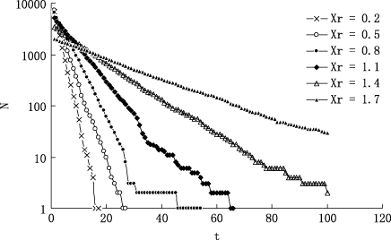
Figure 2. Semi-logarithmic plot of N (the number of time intervals (Δt2 in figure 1) longer than t) versus t for the normal Gaussian distribution signal X (figure 1) for different values of Xr.
Download figure:
Standard image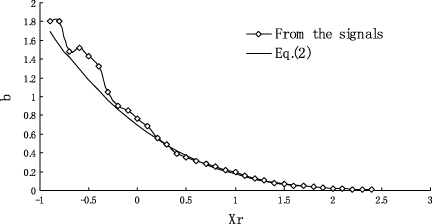
Figure 3. The relationship of b versus Xr.
Download figure:
Standard imageSeismologists have used the statistical properties of the time intervals between successive earthquakes to predict when the next major earthquake will occur [1, 2, 4, 5, 7, 19]. Both the exponential equation and the Weibull equation were found to describe the time interval distribution of earthquakes for different sets of earthquake data. Using a similar approach, we propose that the time interval distribution of sand–dust storms may also be regressed as the Weibull equation

where N is the number of sand–dust storm time intervals lasting longer than t, C and K are constants, and N0 is the total number of time intervals.
To compare the two types of regression equation (equations (1) and (3)) the correlation indices of the curved regression were calculated. The correlation index R2 [3] is defined by
where  is the variance of the observed N values about the best-fitting curved line and
  is the variance of the data points N.
3. Experimental data
Sand–dust storm data recorded in Yanchi, in China, for every spring from 1958 to 2000, were analysed to verify whether the time interval distribution of the sand–dust storms agrees with that of equation (1). Yanchi station (figure 4), which is located in the southern edge of Maowusu Sand Land, has recorded the highest number of sand–dust storms in Loess Plateau of China.
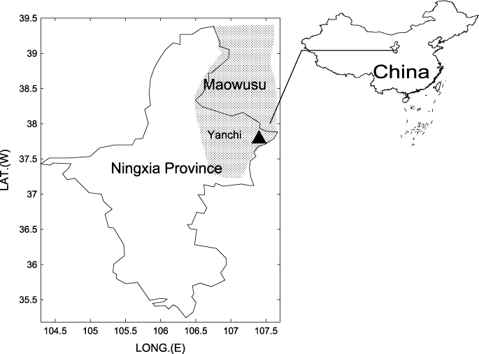
Figure 4. Location of the Yanchi station and Maowusu Sand Land in China.
Download figure:
Standard image4. Results
Figure 5 shows a graph of N versus t/T, wherein the total number of time intervals of sand–dust storms N0 = 539 and the mean time interval of the sand–dust storms T = 4.525 days. (A) and (B) in figure 5 display the same types of data but for different values on the axes. If the regression equation of N versus t matches the exponential equation (equation (1)), the points in (A) should be along a straight line; if the regression equation matches the Weibull equation (equation (3)), the points in (B) should be along a straight line. In figure 5(A), the points form a straight line for t/T < 5, whereas in figure 5(B) all the points form a straight line. From the correlation index R2 shown in table 1, the distribution of time intervals between sand–dust storms for all the spring data is much higher for equation (3), i.e., the Weibull equation N/N0 = exp(−(t/C)K).
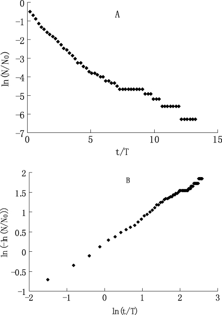
Figure 5. N, the number of time intervals of the sand–dust storms (with length greater than t), against t, from Yanchi spring sand–dust storm data from 1958 to 2000. (A) and (B) show the same data plotted with different values on the axes; if the regression equation matches the exponential equation (equation (1)), the points in (A) should fit a straight line; if the regression equation matches the Weibull equation (equation (3)), the points in (B) should fit a straight line.
Download figure:
Standard imageTable 1. Comparison of the two types of regression equation from figure 4 (equations (1) and (3)) .
| Regression range | Regression equation | Correlation index R2 |
|---|---|---|
| 0 < t/T < 13.3 | N = 156.04 exp(−0.0898t) | 0.7245 |
| N = N0 exp(−(t/3.1867)0.6337) | 0.997 | |
| 0 < t/T < 5 | N = 328.33 exp(−0.1481t) | 0.980 |
| N = N0 exp(−(t/3.3312)0.6667) | 0.996 |
For the time record model (figure 1), the exponential equation for the time interval distribution is based on the assumption that Xr (the normalized threshold wind speed of the sand–dust storm) is constant. However, the threshold wind speed of the sand–dust storms is not constant throughout the year and is lower in spring than in autumn [11]. It is suggested that if the sand–dust storm threshold wind speed were constant, the time interval distribution of the sand–dust storms would agree with the exponential equation rather than the Weibull equation. Figure 6 is similar to figure 5; however, the sand–dust storm data set used in figure 6 is that for only April in the period of 1958–2000. T is 2.78 days, which is less than the value for the entire spring period (4.525 days). For the April sand–dust storm data, the correlation index R2 (figure 6) of the time interval distribution of sand–dust storms shows a better fit to the exponential equation (equation (1)).
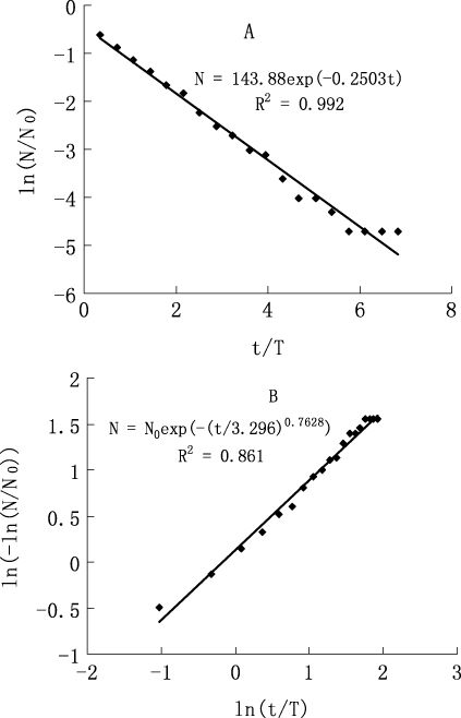
Figure 6. Similar to figure 5; the sand–dust storm data set used in this figure is that for only April and with an N0 of 224 and a T of 2.78 days. The regression function of equations (1) and (3) and the correlation index R2 are also shown.
Download figure:
Standard image5. An explanation for the experiment results
From the time record model of figure 1, the Weibull equation for the time interval distribution can also be obtained for Xr, which varies with time. Figure 7 shows the variation of N with time t when Xr also varies with time. The Xr = 1.7 + sin(25.1t/50 000) and 1.7 + 0.5 sin(25.1t/50 000) time interval distributions fit the Weibull equation, while the Xr = 1.7 time interval distribution fits the exponential equation. So we believe that the variation of the threshold of the sand–dust storm wind speed in spring causes the sand–dust storm time interval distribution in spring to favour the Weibull equation rather than the exponential equation.

Figure 7. Similar to figure 2. ('Xr = 1.7 + sin(25.1t/50 000)' and 'Xr = 1.7 + 0.5 sin(25.1t/50 000)' represent the examples where Xr varies with time t. Their periods are both 12 500 (=50 000 × 2π/25.1). Their amplitudes are 1 and 0.5 respectively. 'Xr = 1.7' represents the example where Xr does not vary with time t.)
Download figure:
Standard image6. Conclusion and discussion
We investigated the distribution of time intervals between spring sand–dust storms recorded in Yanchi, China. For the spring sand–dust storm data recorded from 1958 to 2000, the time interval distribution of sand–dust storms shows a better fit to the Weibull equation N/N0 = exp(−(t/C)K) than to the exponential equation N = Aexp(−bt). However, considering only the April sand–dust storm data, the time interval distribution of sand–dust storms fits the exponential equation rather than the Weibull equation.
For the time record model (figure 1), varying the threshold of the sand–dust storm wind speed in spring causes the sand–dust storm time interval distribution in spring to favour the Weibull equation rather than the exponential equation. This study also suggests that the sand–dust storm threshold wind speed can be taken as a constant over the period of April but not over the entire spring period for Yanchi station. The physical model of figure 1 may help to explain the distribution models for time intervals between successive earthquakes and utilize earthquake time records in earthquake forecasting.
This study brings up two new ideas, which are (1) to mine the information regarding the sand–dust storm threshold wind speed from an exponential sand–dust storm time interval distribution, and (2) to test the above characteristics of time interval distributions for the sand–dust storm data from other stations.