


Abstract
Predicting strains, stresses and swelling in nuclear power plant components exposed to irradiation directly from the observed or computed defect and dislocation microstructure is a fundamental problem of fusion power plant design that has so far eluded a practical solution. We develop a model, free from parameters not accessible to direct evaluation or observation, that is able to provide estimates for irradiation-induced stresses and strains on a macroscopic scale, using information about the distribution of radiation defects produced by high-energy neutrons in the microstructure of materials. The model exploits the fact that elasticity equations involve no characteristic spatial scale, and hence admit a mathematical treatment that is an extension to that developed for the evaluation of elastic fields of defects on the nanoscale. In the analysis given below we use, as input, the radiation defect structure data derived from ab initio density functional calculations and large-scale molecular dynamics simulations of high-energy collision cascades. We show that strains, stresses and swelling can be evaluated using either integral equations, where the source function is given by the density of relaxation volumes of defects, or they can be computed from heterogeneous partial differential equations for the components of the stress tensor, where the density of body forces is proportional to the gradient of the density of relaxation volumes of defects. We perform a case study where strains and stresses are evaluated analytically and exactly, and develop a general finite element method implementation of the method, applicable to a broad range of predictive simulations of strains and stresses induced by irradiation in materials and components of any geometry in fission or fusion nuclear power plants.
Export citation and abstract BibTeX RIS

Original content from this work may be used under the terms of the Creative Commons Attribution 3.0 licence. Any further distribution of this work must maintain attribution to the author(s) and the title of the work, journal citation and DOI.
1. Introduction
One of the challenges associated with the design, construction and operation of a fusion or an advanced fission power plant is the need to predict stresses, strains, and swelling resulting from the exposure of structural components of a reactor to irradiation during operation [1–5]. These stresses and strains have a microscopic origin and stem from the fact that radiation defects have substantial elastic relaxation volumes [6, 7], which give rise to strong local deformation of the lattice. For example, the elastic relaxation volume of a self-interstitial atom defect in tungsten, predicted by density functional theory, is  , where
  is the volume of an atom, whereas the relaxation volume of a vacancy is
  , see e.g. [7, 8]. The large positive mismatch between elastic relaxation volumes of self-interstitial and vacancy type defects in metals, which accumulate in the microstructure as a result of irradiation, gives rise to the local volumetric expansion, and produces stresses in materials exposed to irradiation, resulting in macroscopic swelling and heterogeneous deformation of reactor components.
Models for swelling developed since the 1970s focus on one particular aspect of the phenomenon, the diffusion-mediated preferential absorption of self-interstitial atom defects by dislocations [6, 9–11]. There is extensive literature on the dynamics of accumulation of defects in microstructure and particularly on the evaluation of dislocation bias factors [6, 12–17], which are then used as input parameters for mean-field rate theory models describing the dynamics of growth of voids in materials exposed to irradiation [9–11, 18]. These mean-field models do not require, and do not evaluate, the macroscopic stresses and strains resulting from the accumulation of defects. Neither do they take into account the fact that elastic relaxation of complex defect configurations involves the accumulation of very strong local deformation of the lattice near the defects, with a consequence that the relaxation volume of a complex defect cluster is not equal to the sum of relaxation volumes of constituting defects. The defect configurations formed in collision cascades initiated by high-energy neutrons [19–24] have a fairly complex structure, and their relaxation volumes, and local strains and stresses are sensitive to the relative proximity of individual defects.
A particularly significant practical aspect of the problem of accumulation of radiation defects in structural materials exposed to high-energy neutron irradiation during power plant operation, which has so far eluded a satisfactory solution, is related to the fact that in a treatment of deformation of a component exposed to irradiation, not only the presence of defects in the bulk of the material, but also boundary conditions at surfaces, define the final configuration of stresses and strains. For example, it is known that the magnitude of the total elastic relaxation volume of a point defect depends on boundary conditions at surfaces of the material where it resides and, surprisingly, the role of boundary conditions does not diminish in the macroscopic limit [25, 26].
Below we develop a real-space multi-scale model for strains and stresses produced in reactor components by spatially distributed complex configurations of radiation defects produced by irradiation. We show that if the properties of materials are reasonably isotropic, it is the defect relaxation volume density, i.e. the real-space distribution of relaxation volumes of self-interstitial and vacancy defects and clusters of such defects in a reactor component, that fully defines the resulting macroscopic strains and stresses. Individual defects and clusters of defects act as sources of strains and stresses, which are determined self-consistently, taking into account the appropriate boundary conditions. The fundamental notions relating macroscopic strains and stresses to microstructure are the dipole tensor and relaxation volume of a defect object, which can be an individual point defect or a large cluster of such defects formed in a collision cascade. We show that the dipole tensor of a defect, which has so far only been applied to nano-scale point defects [7, 25, 27], can in fact be used for characterizing defect objects of arbitrary size. This is a mere consequence of the fact that there is no characteristic spatial scale in elasticity equations. At a large distance from an arbitrarily complex configuration of defects, for example, a cluster of defects containing thousands of individual point defects, the elastic strain generated by the cluster equals
where  is the position of the defect cluster,
  is Green's function of elasticity equations [28], and Pkl is the dipole tensor of the defect configuration. Equation (1) fully defines the strain field generated by a defect cluster at distances that are much greater than its characteristic spatial extent.
It is well established how to compute elastic dipole tensors of point defects [7, 27, 29]. Below, we show how elastic dipole tensors can be defined and evaluated for defect clusters produced by the collapse of entire high-energy collision cascades. The condition that makes it possible to apply the dipole tensor concept to the treatment of strains and stresses in a reactor component is that the spatial scale of a defect object in the radiation-induced microstructure is always small in comparison with the spatial scale of a component.
Historically, elastic dipole tensors were introduced in order to treat long-range elastic fields of nano-scale point defects, and elastic interactions between such defects, as well as between defects and dislocations [25, 30, 31]. Still, the fact that the universal scale-free nature of elasticity equations enables extending the notion of elastic dipole tensor of a defect to mesoscopic and macroscopic scales, does not appear to have been recognized.
In the treatment of a spatially-localized defect configuration, which may include defects produced by the collapse of an entire cascade or even a group of cascades, it is only necessary to take into account the discreteness of the atomic lattice in the most strongly distorted core regions of defect structures. At large distances from a defect configuration, lattice discreteness is no longer significant and the rate of variation of atomic displacements as a function of spatial coordinates is small  . In this limit, the strain and stress fields generated by a defect configuration are fully characterized by a symmetric
  tensor Pkl. The volume dipole tensor density, and the density of relaxation volumes of defects, vary from one point in the material to another, depending on the local degree of exposure of a material to irradiation. The dipole tensor can be defined independently of the nature of a defect object, for example, it can be defined for a point defect, a dislocation loop [7, 27, 31], or a fairly complex configuration of atomic displacements produced by a collision cascade as a whole. In the latter case, although the volume of the spatial region involved in the calculation of Pkl contains a large number of atoms, it is still small in comparison with the size of a reactor component, justifying the fundamental approximation on which equation (1) is based.
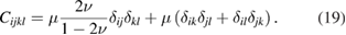
In the next section we outline the formalism involved in the evaluation of stress and strain fields associated with spatially distributed defect structures. We derive the fundamental equations defining strains, stresses and displacements in an arbitrary volume of a material containing spatially distributed defects. If the material is elastically isotropic and defects have no preferred orientation, the strains and stresses are fully determined by the distribution of spatially-varying density of elastic relaxation volumes, a dimensionless function that acts as a source term in equations for the irradiation-induced stresses and strains. Then we show how the relaxation volumes of individual point defects can be computed using ab initio density functional theory methods, and provide accurate values of relaxation volumes computed for several metals with cubic crystal structure. Subsequently, we compare accuracy of ab initio and atomic relaxation methods using semi-empirical interatomic potentials, and show how to obtain accurate values of dipole tensors for entire configurations of defects produced by the collapse of collision cascades initiated by high-energy neutrons. For both cases, we discuss a practical way of defining the density of relaxation volumes of defects and relate it to a measure of exposure of a material to neutron irradiation. We then give a comprehensive derivation of the macroscopic elasticity equations including the density of body forces associated with the accumulation of defects, and provide a full exact solution of these equations for the case of a spherical shell with a source of irradiation at its centre. The solution makes it possible to determine swelling, strains and stresses everywhere in the shell, and it also illustrates the pivotal part played by the boundary conditions for the elasticity equations. Finally, we discuss a finite element implementation of the method and examine a possible application of our approach to the in silico evaluation of operational performance of a fusion power plant.
2. General methodology
At a large distance from a strongly deformed atomic configuration, for example a defect or a cluster of defects, the field of displacements of atoms from their equilibrium positions in the lattice is given by the equation [25]
In this equation, Pkl is the elastic dipole tensor of the defect configuration that, according to (2), fully defines the elastic field that the configuration generates in the material.  is the elastic Green's function [28], which in the isotropic elasticity approximation has the form

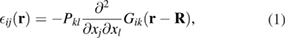
Here, μ is the shear modulus of the material and ν is the Poisson ratio, see [32]. From (2) and (3) we find
where summation over repeated indexes is assumed, and  .
.
Equations similar to (4) have been extensively explored in connection with the treatment of elastic fields of point defects on the nano-scale [7, 27, 33, 34]. However, as the form of equation (4) suggests, there is no specific spatial scale at which it should be applied, as elastic fields have no intrinsic spatial scale associated with them. For example, using formula (4) one can approximate the elastic field of a fairly large defect structure just as easily as one can do this for a point defect.
The magnitude and the angular anisotropy of elastic field is described by the matrix elements of tensor Pkl, which can be evaluated using atomistic simulations with periodic boundary conditions, using the equation [7, 25, 29]
where  is the volume of the simulation cell containing the defect structure, and
  is the volume average stress tensor. In the literature [25, 29], equation (5) has so far been only applied to point defects, and hence the size of the cell used in simulations was relatively small, in most cases not exceeding 103 atoms. However, since the notion of the dipole tensor defined above is entirely general, equation (5) can be applied to a defect structure of arbitrary size, potentially involving millions of atoms and many individual point defects and clusters of defects.
It is convenient to represent Pkl in the following form

where  is an auxiliary
  tensor, also uniquely characterizing the defect structure, and Cijkl is the tensor of elastic constants. The advantage that this representation offers is that it provides a simple and robust way of computing the relaxation volume of an arbitrary complex defect configuration as a whole. Indeed, the relaxation volume of a defect configuration in a body with surfaces free of tractions equals [25]

where  is the elastic compliance tensor [35]. Tensor
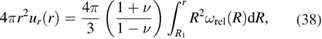
  can be expressed in terms of its eigenvectors and eigenvalues as
where eigenvectors  form a mutually orthogonal set, and eigenvalues
  have the meaning of partial relaxation volumes. They satisfy the condition
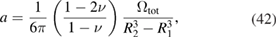
which, if the defect configuration has been formed as a result of a collision cascade event initiated by an energetic neutron, gives the total relaxation volume of cascade debris. Swelling, often occurring under neutron irradiation, results from the accumulation of uncompensated relaxation volumes of defects and defect clusters produced in collision cascades initiated by neutrons.
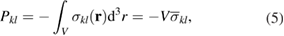
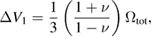
In engineering applications, where the scale of effective volumes containing defects is large, and defects and defect clusters adopt random spatial orientations, the eigenvectors of tensor  may point in any spatial direction with equal probability. For example, consider the relaxation volume tensor of a crowdion defect [7] shown schematically in figure 1


Figure 1. A sketch of a self-interstitial crowdion defect, where the axis of the defect is parallel to the ![$[1\, 1\, 1]$](https://content.cld.iop.org/journals/0029-5515/58/12/126002/revision4/nfaadb48ieqn019.gif) crystallographic direction.
crystallographic direction.
Download figure:
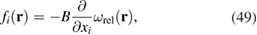
Standard image High-resolution imageThe direction vector  of the axis of the defect can adopt any of the four
  type directions. As a result, the average over defect orientations relaxation volume tensor is diagonal with respect to m and n.
Similarly, we can define an average over orientations for the relaxation volume tensor of a complex defect
Here  denotes averaging over all the directions in the solid angle of
  , namely
For a unit vector in 3D space  we find that

and
Substituting this into equation (6) we arrive at
which for crystals of cubic symmetry becomes
In the isotropic elasticity limit the above equation for the dipole tensor reduces to [7, 31]
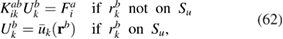
where B is the bulk modulus of the material.
In applications, where macroscopic elastic fields are formed as a result of superposition of microscopic fields created by millions of individual defects and defect clusters, which all adopt arbitrary orientations in the lattice, it is often sufficient to use the above isotropic approximation for the dipole tensor. The advantage offered by this approximation is that a defect object is characterized by only one parameter, its relaxation volume  . In some cases, for example in crystals with non-cubic symmetry or in the presence of significant external anisotropic elastic strain field, it may prove necessary to take into account the anisotropy of defect structures.
The field of elastic displacements generated by a defect object, the dipole tensor of which has the form (16), equals
The strain field, corresponding to this field of displacements, is
To compute the elastic stress associated with the strain field given by (18), we need to multiply the strain tensor by the four-index tensor of elastic constants, which in the isotropic elasticity approximation equals [26]
The resulting expression for the stress field generated by a defect object at  is
is

We now define the central notion of our treatment, the density of relaxation volumes of defects, which is a dimensionless quantity equal to the total relaxation volume of all the defect configurations in a unit volume of material
where summation is performed over all the defect clusters a in the material. Because of the properties of the Dirac delta-function, if we integrate  over a certain volume element in the material, only the defect clusters contained in that volume element are going to contribute to the integral. There is a fundamental relation between the notion of the number of displacements per atom [36], which is a measure of exposure of a material to irradiation, and the density of relaxation volumes of defects that such exposure produces. Below, we show that function
  provides a quantitative measure of the magnitude of sources of stresses and strains produced in materials by radiation defects.
A quantity similar to (21) was introduced by Caturla et al [37, 38] in the context of modelling microstructural evolution and swelling of materials under irradiation. To explain swelling, in [37, 38] the density of relaxation volumes of vacancies was taken as a positive quantity. This does not agree with ab initio calculations, showing that vacancies have negative relaxation volumes whereas self-interstitial atom defects have positive relaxation volumes. Swelling results from the agglomeration of self-interstitial defects into dislocation loops and extended dislocation network; vacancies aggregate into voids, the relaxation volume of which in the macroscopic limit is negative and small [39].
The elastic strain, generated by all the defects produced by irradiation and distributed with certain density in the bulk of a reactor component, can be computed by integrating the point source function (18) with the density of relaxation volumes of defects (21) as

We note that equation (18) follows from (22) if we assume  .
.
Computing the stress generated in a material by a continuous distribution of defects involves an element of mathematical subtlety. First, we re-write equation (22) in the form
To find the elements of the stress tensor

we multiply (23) by the four-index tensor of elastic constants (19). This gives
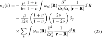
where the second term, proportional to  , arises from the first term in (19). Noting that
we find the stress produced by a continuous distribution of defects
The density of body forces arising from a continuous distribution of defects can now be found by differentiating the stress tensor with respect to xj, namely [40]
Deriving the first term in the above equation involved integration by parts
The addition of the two terms in (27) gives the density of body forces resulting from the accumulation of defects in the material
This equation is one of the key findings of this work.
For completeness, we also note the expression for the field of elastic displacements produced by the defects distributed in the bulk of a reactor component with relaxation volume density (21), namely
Equations (22)–(25) fully define the elastic field generated directly by the sources of stresses and strains associated with relaxation volumes of spatially distributed radiation defects. However, these equations do not take into account the boundary conditions at surfaces, which give a surprisingly large contribution to the observed strains, stresses, and swelling. It is known that in the treatment of elastic fields of point defects, strains and stresses associated with boundary conditions have the same magnitude as strains and stresses (22)–(25) generated by the defects themselves, see for example [25, 26]. Below we show that, for example, in tungsten only 59% of the observed swelling comes directly from the sources in the integral equations representing relaxation volumes of defects. The remaining 41% of the swelling effect comes from strains and stresses associated with boundary conditions.
In the next section we describe how function  can be computed or estimated using ab initio methods and molecular dynamics simulations, and generic assumptions about the spatial distribution of radiation damage. We then investigate the case of a spherical shell containing an isotropic neutron source, representing for example a vacuum vessel of a fusion power plant or the casing of a fissile fuel element, and solve the above equations for the stress and strain analytically. We then develop a finite element implementation of the approach described above, to enable computing strains and stresses in components of arbitrary shape and size exposed to irradiation.
3. Relaxation volumes of point defects in bcc transition metals and gold
In this section we summarize results of ab initio density functional theory calculations of relaxation volumes of self-interstitial atoms (SIA) and vacancy defects in several bcc transition metals and in gold. The availability of such data is still relatively limited as the majority of density functional calculations of defects performed so far focused on the accurate evaluation of energies of defects [42–45], rather than on the evaluation of elastic properties of defects [7, 8, 27, 29, 46]. The relaxation volume of a Frenkel pair can be approximated by the sum of relaxation volumes of an SIA and a vacancy. In non-magnetic bcc transition metals, the  dumbbell is the most stable SIA defect configuration [47]. We have evaluated the relaxation volumes of SIA and vacancy defects in vanadium, niobium, molybdenum, tantalum and tungsten using equation (5). DFT calculations were performed using the approach described in [7]. Relaxation volumes of vacancies were computed using simulation boxes containing
  bcc unit cells, using a
  k-point mesh and the GGA-PBE functional.
Results of ab initio calculations of relaxation volumes of defects are summarised in table 1. The relaxation volume of a vacancy is negative whereas the relaxation volume of a SIA defect is positive, and in most cases larger than the volume of an atom. The data given in the table show that the relaxation volume of a Frenkel pair is close to one atomic volume. Relaxation volumes of point defects in fcc gold (Au) were evaluated in [41]. In gold, the most stable configuration of a SIA defect is a  dumbbell. The relaxation volume of a Frenkel pair in gold is close to 1.64 atomic volume, larger than in bcc transition metals.
Table 1. Relaxation volume of  self-interstitial atom (SIA) dumbbell defects and vacancies in non-magnetic bcc transition metals, and of a
  self-interstitial dumbbell defect and a vacancy in fcc gold. The relaxation volume of a Frenkel pair is approximated by the sum of relaxation volumes of a SIA defect and a vacancy. Data are given in atomic volume units; defect relaxation volumes in gold are taken from [41].
 |
 |
 |
|
|---|---|---|---|
| V | 1.472 | −0.493 | 0.979 |
| Nb | 1.554 | −0.405 | 1.149 |
| Mo | 1.538 | −0.353 | 1.185 |
| Ta | 1.524 | −0.410 | 1.114 |
| W | 1.712 | −0.345 | 1.367 |
| Au | 2.02 | −0.38 | 1.64 |
4. Validation of MD data against DFT calculations
To compare defect dipole tensors computed using semi-empirical many-body interatomic potentials with ab initio results derived from density functional calculations, we evaluated dipole tensors of point defects in tungsten.
All the ab initio calculations were performed using Vienna Ab initio Simulation Package (VASP) [48–51]. We used the PBE [52, 53] and AM05 [54–56] exchange-correlation functionals. The plane wave energy cutoff was 450 eV. We used a supercell containing  bcc unit cells, and a
  k-points mesh. First, we created perfect lattice cells containing 128 atoms and fully relaxed them, to find the equilibrium lattice parameter. Then, we created cells containing point defects. Ionic positions were relaxed, but the cell size and shape remained the same as in the perfect lattice case. Elastic dipole tensors were computed from macro-stresses using equation (5). The computed values are given in tables 2 and 3.
We have also evaluated dipole tensors of point defects using molecular statics and semi-empirical interatomic potentials. We used the Marinica (EAM4) [57] and DND potentials [47]. Similarly to ab initio calculations, we first fully relaxed a simulation box containing  perfect bcc unit cells. Then, we inserted or removed atoms in the cell, creating point defects. This was followed by the relaxation of atomic configurations, where again we did not change the cell size and shape. The dipole tensors were computed using equation (5). The computed values are given in tables 4 and 5. Comparison of elements of dipole tensors computed using density functional theory and semi-empirical potentials in tables 2–5, show that whereas the results agree qualitatively, there are significant differences between the absolute values. This is perhaps not surprising since the main criterion used in fitting the semi-empirical potentials to ab initio data has been the agreement between the energies of atomic configurations. Elastic properties of defects have so far received relatively little attention although, as we show in this study, they play a pivotal role in determining the magnitude of strains and stresses in reactor components under irradiation.
To evaluate the density of relaxation volumes of radiation defects (21), it is not enough to know the number of Frenkel pairs per unit volume. It is only in the limit where self-interstitial atom defects and vacancies are distributed randomly as an ideal gas of defects that the density of relaxation volumes can be estimated as

where  and
and  are the volume densities of self-interstitial atom and vacancy defects, and where the relaxation volume of a SIA defect
  is positive and the relaxation volume of a vacancy
  is negative.
If defects form clusters, for example dislocation loops or voids, the relaxation volume of a cluster of defects is different from the sum of relaxation volumes of defects forming the cluster. For example, the volume of a dislocation loop in the macroscopic limit equals the scalar product of its Burgers vector and its vector area  , and can be positive or negative, depending on the interstitial or vacancy character of the loop [7, 31]. The relaxation volume of a void, which is a large cluster of vacancies, vanishes in the macroscopic limit [39]. The relaxation volume of a vacancy-helium cluster depends on the relative number of vacancies and helium atoms in a cluster [8].
In the next section we evaluate relaxation volumes of clusters of defects formed in collision cascades. We show that the total relaxation volume of cascade debris is still proportional to the number of Frenkel pairs produced in a cascade event, however it is not given by equation (31) above.
Table 2. Elastic dipole tensors of point defects in tungsten. The values were computed using density functional theory with the PBE exchange-correlation functional. All the values are in eV units.
| PBE | P11 | P22 | P33 | P12 | P23 | P31 |
|---|---|---|---|---|---|---|
| 100dumbbell | 65.92 | 53.38 | 53.38 | 0.00 | 0.00 | 0.00 |
| 110dumbbell | 56.96 | 52.56 | 52.56 | 0.00 | 11.28 | 0.00 |
| 111crowdion | 52.74 | 52.74 | 52.74 | 13.15 | 13.15 | 13.15 |
| 111dumbbell | 52.75 | 52.75 | 52.75 | 13.13 | 13.13 | 13.13 |
| Octa | 52.74 | 52.74 | 67.21 | 0.00 | 0.00 | 0.00 |
| Tetra | 47.36 | 59.11 | 59.11 | 0.00 | 0.00 | 0.00 |
| Vacancy | −9.98 | −9.98 | −9.98 | 0.00 | 0.00 | 0.00 |
Table 3. Elastic dipole tensors of point defects in tungsten. The values were computed using density functional theory and the AM05 exchange-correlation functional. All the values are in eV units.
| AM05 | P11 | P22 | P33 | P12 | P23 | P31 |
|---|---|---|---|---|---|---|
| 100dumbbell | 66.34 | 53.85 | 53.85 | 0.00 | 0.00 | 0.00 |
| 110dumbbell | 57.37 | 53.71 | 53.71 | 0.00 | 11.77 | 0.00 |
| 111crowdion | 53.84 | 53.84 | 53.84 | 13.24 | 13.24 | 13.24 |
| 111dumbbell | 53.84 | 53.84 | 53.84 | 13.22 | 13.22 | 13.22 |
| Octa | 53.26 | 53.26 | 68.30 | 0.00 | 0.00 | 0.00 |
| Tetra | 48.13 | 59.93 | 59.93 | 0.00 | 0.00 | 0.00 |
| Vacancy | −10.95 | −10.95 | −10.95 | 0.00 | 0.00 | 0.00 |
Table 4. Elastic dipole tensors of point defects in tungsten. The values given in this table were computed using the Marinica (EAM4) semi-empirical interatomic potential for tungsten. All the values are in eV units.
| Marinica | P11 | P22 | P33 | P12 | P23 | P31 |
|---|---|---|---|---|---|---|
| 100dumbbell | 49.85 | 40.12 | 40.12 | 0.00 | 0.00 | 0.00 |
| 110dumbbell | 52.91 | 53.69 | 53.69 | 0.00 | 13.24 | 0.00 |
| 111crowdion | 35.16 | 35.16 | 35.16 | 14.82 | 14.82 | 14.82 |
| 111dumbbell | 37.16 | 37.16 | 37.16 | 16.59 | 16.59 | 16.59 |
| Octa | 45.10 | 45.10 | 59.77 | 0.00 | 0.00 | 0.00 |
| Tetra | 48.02 | 49.94 | 49.94 | 0.00 | 0.00 | 0.00 |
| Vacancy | −1.07 | −1.07 | −1.07 | 0.00 | 0.00 | 0.00 |
Table 5. Elastic dipole tensors of point defects in tungsten. The values given in this table were computed using the Derlet–Nguyen-Manh–Dudarev (DND) semi-empirical interatomic potential for tungsten. All the values are in eV units.
| DND | P11 | P22 | P33 | P12 | P23 | P31 |
|---|---|---|---|---|---|---|
| 100dumbbell | 55.70 | 23.49 | 23.49 | 0.00 | 0.00 | 0.00 |
| 110dumbbell | 32.60 | 33.97 | 33.97 | 0.00 | 3.70 | 0.00 |
| 111crowdion | 36.98 | 36.98 | 36.98 | 13.64 | 13.64 | 13.64 |
| 111dumbbell | 38.21 | 38.21 | 38.21 | 13.65 | 13.65 | 13.65 |
| Octa | 25.54 | 25.54 | 60.66 | 0.00 | 0.00 | 0.00 |
| Tetra | 18.15 | 43.65 | 43.65 | 0.00 | 0.00 | 0.00 |
| Vacancy | −3.33 | −3.33 | −3.33 | 0.00 | 0.00 | 0.00 |
5. Evaluation of dipole tensors of defects and clusters of defects by atomistic calculations
5.1. The dipole tensor for a large, complex defect
Equation (2) gives the displacement field at a position  , which is sufficiently far away from a defect so it can be treated as a point source of elastic deformation. If there are m such point sources, the displacement field at
  is simply the sum over their contributions. Contributing point sources could be a substitutional atom whose local environment induces a stress upon it, but equally could be a point defect, or a cluster of defects, viewed from a distance. The dipole tensor of a large, complex defect therefore has the same simple physical interpretation as that of a point defect or a small defect cluster—it can be approximated by a point source of stress which produces the same displacement field (to leading order) as the sum of its contributing parts.
We can say that a complex defect is a group of m contributors, where the  th contributor has dipole tensor
  and position
  . We would like to represent this with a single dipole tensor Pkl at position
  . The displacement at
  due to the group of m contributors is
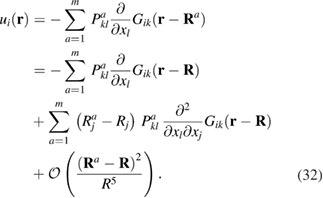
We recognize the first term as the displacement field due to a single defect of strength  at
at  , and the second term as the first-order correction due to the spatial extent of the defect. The spherical average of the second derivative of Gik is zero, so to minimise the second term we choose
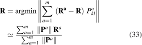
where 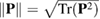 is the Frobenius norm, used here as a measure of the strength of the ath contributor. In this way we can define a single dipole tensor and single position for a complex defect.
5.2. Dipole tensor for defects generated by a collision cascade
In this section we compute the dipole tensors for collision cascades in bulk tungsten simulated with classical molecular dynamics. It is not our intention here to provide an exhaustive database of values of dipole tensors, only to describe the relative ease of such a calculation. For an empirical potential we can define the energy as a sum over all atoms a, and so [58]
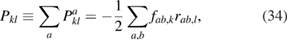
where fab,k is the kth Cartesian component of the force acting on atom a due to atom b and rab,l is the lth Cartesian component vector separation between them. The second derivative of energy with respect to strain gives the (fourth-rank) elastic constant tensor, needed for evaluating the relaxation volume given by equation (7).
Collision cascades were simulated with the classical molecular dynamics code PARCAS. A simulation supercell of 6.8 million atoms at 0 K was established with periodic stress-free boundary conditions, then a cascade was initiated by giving a single atom a large kinetic energy (100 keV–200 keV) in a random direction. The DND interatomic potential for tungsten by Derlet et al [47], stiffened at short range by Björkas et al [59], was used for the simulations, and a non-local friction force was applied to atoms with a kinetic energy above 10 eV to account for energy loss due to electronic stopping [60]. A Berendsen thermostat [61] set to 0 K was applied to the atoms in a 1.5 unit cell thick region along all periodic boundaries. Cascades were followed for 40 ps, at which point further defect evolution is thermal rather than ballistic. Details of the simulation method can be found in [20]. Similar cascade simulations have been shown to reproduce the observed experimental cluster size-frequency distribution [21, 23] and spatial extent [24]. A typical relaxed cascade configuration is shown in figure 2. To compute the dipole tensor for the atomically relaxed configuration, the atoms in the supercell could in principle be directly relaxed with conjugate gradients or a similar method, but in practice we have found that the dipole tensor converges rather slowly in a large box, and a standard convergence criterion based on force-per-atom or total energy difference alone may return without a well-converged dipole tensor. Instead we take the calculation as a three-stage procedure: first the atoms deviating more than  lattice parameter from crystal positions were identified, and a buffer of four unit cells in all directions was added. A smaller rectangular cell containing these atoms was cropped from the cascade and fully relaxed. At this point the dipole tensor is converged to within 10%. The smaller cell was then re-embedded into a 4 million atom perfect crystal supercell (
 unit cells), and relaxed again. The dipole tensor is computed after the second relaxation. Finally the dipole tensor computed for the perfect crystal lattice at the original supercell size was computed and subtracted—this may not be exactly zero if the lattice parameter is only specified to a fixed precision, and needs removing as it scales with system size. We find convergence in the dipole tensor to better than 1% precision after a few hours cpu time. We expect this precision to be significantly better than the accuracy of the potentials or the description of the cascade structure.
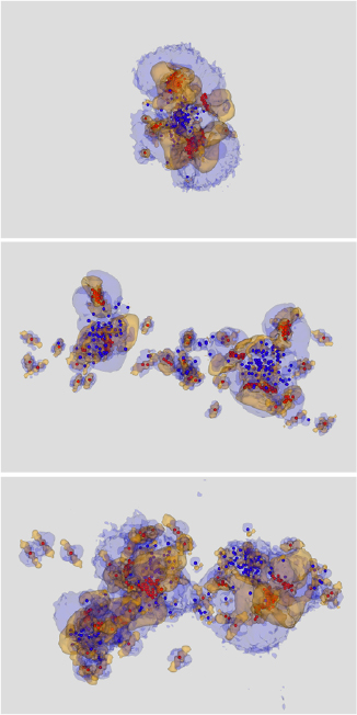
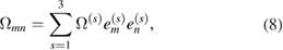
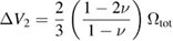
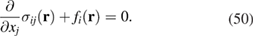
Figure 2. Typical high-energy displacement cascades in tungsten, evolved to 40 ps and then atomically relaxed at constant volume. The initial energies of recoil atoms giving rise to a cascade event: top to bottom: 100 keV PKA, 150 keV, 200 keV. Vacancies (blue) and interstitials (red) have been identified using a Wigner–Seitz cell analysis. The defect clusters introduce both compressive and rarefactive stresses. Yellow isosurfaces show the region where atoms contribute Tr(P) = +0.15 eV per atom to the dipole tensor (compressive stress), blue isosurfaces where Tr(P) = −0.05 eV per atom (rarefactive) computed using equation (34). Details of these simulations are given in the text and table 6. The classic cascade structure of vacancy-rich core surrounded by interstitial clusters can be observed. From a distance, the structure of the cascade is immaterial, and the long-range elastic field of the cascade can be computed from a single dipole tensor capturing the sum of the contributions from each defect cluster formed in a cascade. Images rendered using Ovito [62].
Download figure:
Standard image High-resolution imageTable 6. Results for the dipole tensor for three representative displacement cascades simulated using molecular dynamics. The energy of the initial primary knock-on atom (PKA) is given in kiloelectron-Volts (keV), the number of Frenkel pairs was computed by the Wigner–Seitz cell analysis of the final cascade configuration. The partial relaxation volumes were computed using equation (8). The total relaxation volume of a cascade is also reported as a multiple of the volume per atom,  . Elements of dipole tensors and relaxation volumes are converged to better than 1%.
| PKA energy (keV) | 100 | 150 | 200 |
|---|---|---|---|
| Number of Frenkel pairs | 199 | 174 | 198 |
| Elements of the dipole tensor (eV) | |||
| P11 | 2340 | 3080 | 3640 |
| P22 | 1480 | 2860 | 3410 |
| P33 | 2030 | 2450 | 3140 |
| P23 | −907 | 62 | −1420 |
| P31 | −1580 | −335 | 351 |
| P12 | −367 | 1700 | −714 |
Partial relaxation volumes  ( ( ) ) |
|||
 |
−1570 | −1150 | −908 |
 |
505 | 331 | 2220 |
 |
2040 | 2220 | 2240 |
Relaxation volumes  |
61.4 | 88.2 | 107.0 |
Dipole tensors were computed for isolated defects and relaxed cascade configurations using the stress method, equation (5). Results for idealised isolated defects are given in section 4, from which we conclude that empirical potentials give reasonable results. We note that the relaxation volume for a single tungsten SIA is around 1.7  , but for a large loop containing N interstitials the relaxation volume drops to
  , in agreement with elasticity analysis [7, 31]. Defect dipole tensors for the full cascades are given in table 6. We conclude that the relaxation volume of a cascade scales with the number of Frenkel pairs, with the DND potential giving

The elastic relaxation volume density  of cascades resulting from atomic recoils of energy E can be computed as
where  is the spatial density of cascades with energy E and
  is the relaxation volume of defects produced in a cascade initiated by a recoil atom of energy E. In practice, this function can be computed using neutron transport calculations for a realistic reactor geometry [63, 64] followed by the evaluation of local spectra of primary knock-on atoms [65] and the treatment of the subsequent evolution of microstructure, including modelling dislocation climb [66], self-climb [67], and the formation of a network of dislocations, voids and gas bubbles.
6. Strains, stresses and swelling in a spherical shell: an exact solution
Above, we showed how to compute the relaxation volume density (21) using ab initio calculations and molecular dynamics simulations of high energy collision cascades. In this and the next sections we show how to solve the elasticity equations and compute strains, stresses and swelling of components assuming that function  is known. In this section, we show how to solve equations (23)–(30) analytically in the limit where the problem has spherical symmetry, and in the next section we describe a general numerical finite element approach suitable for the treatment of arbitrary configurations.
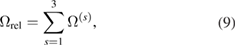
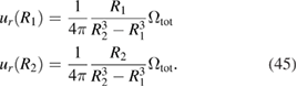
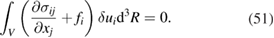
Consider a component, for example the vacuum vessel of a fusion power plant or the cladding of a fuel cell containing fissile nuclear fuel, which we assume has the form of a spherical shell sketched in figure 3.
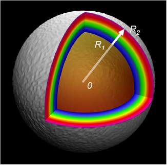
Figure 3. A sketch of a spherical shell containing a source of neutrons in its central part. The solution described in this section gives the distribution of stresses and strains in the material of the shell for  .
.
Download figure:
Standard image High-resolution imageIf the source of neutrons inside the shell is isotropic, then the distribution of defect relaxation volumes in the material depends only on the distance r to the centre of the shell and is independent of the polar and azimuthal angles θ and ϕ of the spherical system of coordinates, the origin of which is at the centre of the shell.
The solution that we are interested in is defined on the interval  , where R1 is the inner radius of the shell and R2 is its outer radius. The field of displacements is radially-symmetric and the vector of displacements can be written as
  , where
  . Differentiating equation (30), we find
The above equation has a simple meaning, namely that it is the density of relaxation volumes of defects that causes the material to expand or contract as a result of accumulation of defects in the material. Note the remarkable prefactor  in the above equation, the numerical value of which is close to 0.6 for tungsten. This prefactor shows that the direct deformation of the lattice caused by the accumulation of defects is only partially responsible for the observed dimensional changes occurring as a result of irradiation. The other, similar in magnitude, contribution comes from the boundary conditions at surfaces, as we prove below.
Since the field of displacements is radially symmetric, we apply the divergence theorem to equation (37) and write
for  .
.
Noting that in the absence of radiation defects the divergence of  is a harmonic function of coordinates [40], we write the field of displacements as a sum of the partial solution of heterogeneous equation (37) and a general solution of the corresponding homogeneous equation, namely
Here a and b are constants that need to be determined from boundary conditions at r = R1 and r = R2. Assuming that pressure at R1 and R2 is negligible in comparison with the stresses developing in the material due to the accumulation of defects, we adopt the traction free boundary conditions [25]  at r = R1 and r = R2.
Strains can be found by differentiating (39). They have the form
To find stresses, we need to multiply the above expression for the strain tensor by the four-index tensor of elastic constants (19). The resulting expression has the form
Applying the traction-free boundary conditions at r = R1 and r = R2 to (41), we find parameters a and b, namely
and
where
is the total relaxation volume of all the defects in the material of the shell.
The total macroscopic change of volume resulting from the accumulation of defects in the materials of the shell is given by the integral of the trace of the full strain tensor (40) over the volume of the component
where we noted that  and
and  . The integration of the first term in square brackets over the volume of the shell gives
whereas the second term in (44), proportional to a and arising from the boundary conditions, contributes
to the total macroscopic swelling of the shell. The sum of these two terms equals  , confirming that swelling is as much an effect of direct expansion of the lattice due to the accumulation of defects in the material, as it is an effect associated with boundary conditions and arising from long-range stresses and strains of defects interacting with the boundaries of the component.
Substituting (42) and (43) into (39), we find radial displacements of the inner and outer surfaces of the shell
These displacements satisfy the condition

which provides an alternative way of evaluating the total volumetric swelling of the shell. A remarkable property of equation (45) is that they show that both the inner and outer surfaces of an irradiated spherical shell relax outwards. The magnitude of surface displacements can be substantial. For example, the surface of a vacuum vessel with the inner radius of R1 = 5 metres, after exposure to neutron irradiation, producing constant homogeneous defect relaxation volume density  % in the material, moves outwards by approximately
  cm.
cm.
We can now find elements of the stress tensor developing in the spherical shell as a result of its exposure to irradiation. The radial diagonal element of the stress tensor is
The circumferential (hoop) components  and
and  of the stress tensors are
Due to the spherical symmetry of the problem, we have  . The above formulae are valid for any distribution of defect relaxation volume density
  in the spherical shell, which is a function of radial variable r.
As the density of defects vanishes in the immediate vicinity of free surfaces, 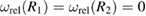 . The radial stress (47) also vanishes at surfaces at r = R1 and r = R2, but the hoop stress (48) remains finite everywhere on the interval
  . The high radial and hoop stresses developing as a result of accumulation of defects in the material are responsible for the loss of structural integrity of the component in the limit where the relaxation volume density of defects exceeds a certain critical level.
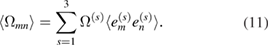
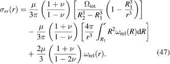
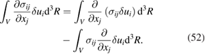
Applications of the above equations to the evaluation of stresses developing in a steel vacuum vessel with inner radius R1 = 3 m and outer radius R2 = 3.5 m as a result of irradiation are illustrated in figure 4. The form of function  used as input reflects the fact that neutron flux from an isotropic source varies as a function of r as
  and also that neutrons are absorbed in steel over a characteristic distance of a fraction of a metre.
Figure 4. Top: two assumed distributions of relaxation volume densities of defects  , referred to as case studies 1 and 2, and their integrals
  in a spherical steel shell with inner radius of R1 = 3 m and outer radius of R2 = 3.5 m. Middle (case study 1) and bottom (case study 2) graphs show radial and hoop stresses in the component computed using equations (47), (48) and FEM using the relaxation volume densities, given in the top graph, as input. The shear modulus of steel is
  GPa,
GPa,  . For comparison, the yield strength of Eurofer97 ferritic-martensitic steel is 530 MPa [68].
Download figure:
Standard image High-resolution imageFigure 4 shows that particularly high stresses develop close to the internal surface of the steel shell even if the amount of damage accumulated in the material is relatively small. The magnitude of radiation-induced stresses can be estimated by evaluating the product of the shear modulus of the material and function  , suitably averaged over the volume of the component.
7. General finite element implementation
In the preceding section, to find analytical solutions for the displacements, strains and stresses in a hollow spherical shell exposed to irradiation, we used equation (30) as a starting point for the analysis. In this section, we develop a general finite element implementation of the method, using which one can evaluate stresses, strains and displacements in any reactor geometry. In the finite element method (FEM), it is more convenient to use the equation for body forces generated by defects (29) rather than the formula for displacements (30). The two approaches are entirely equivalent, as confirmed by the comparison of numerical solutions derived using analytical and FEM implementations for the same reactor geometry and same density of relaxation volumes of defects (see figure 4).
The finite element implementation of the mathematical formalism for computing strains, stresses and swelling of irradiated reactor components developed above, is based on equation (29), which can be written in the form
where ![$B=2\mu(1+\nu)/[3(1-2\nu)]$](https://content.cld.iop.org/journals/0029-5515/58/12/126002/revision4/nfaadb48ieqn100.gif) is the bulk modulus of the material and
is the bulk modulus of the material and  is the density of relaxation volumes of defects (21).
The fundamental equation for the stress tensor, defining the condition of mechanical equilibrium, has the form
To find the displacement field which satisfies (50) using the FEM, this expression for mechanical equilibrium is recast as a virtual work expression [69]; for completeness this is outlined here. Multiplying (50) by an arbitrary displacement field  which satisfies
  on the displacement boundary Su, and integrating over the body
  gives:
Consider the first term
Using the divergence theorem, the first term on the right hand side is
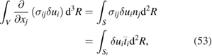
where  are the specified surface tractions on St and by definition the virtual displacement
  on Su and so the surface integral vanishes there. Therefore, after multiplying by −1, (51) becomes
Expressing the stress tensor in terms of displacements,
due to the symmetry of Cijkl. Therefore
This is the expression for virtual work in the presence of a body force fi. This can be discretised and solved at the FE nodes located at  where 1 < a < m, for the unknown displacement at each node
  . The virtual displacement and its derivative are interpolated using the shape functions
The displacement derivative is interpolated in a similar manner, namely
where  is the nodal shape function of node a which satisfies

Substituting (57)–(59) into (56) gives
and as the virtual displacement  is arbitrary, the term in square brackets must be zero. In matrix form, the following system of equations is obtained
where
 is the global stiffness matrix.
  is the global force vector which includes a body force contribution at every node not on Su, and surface traction contribution
  for every node on St. Substituting the body force
  from (49) into (63) gives
The advantage of using the body force is that it has a remarkably simple form (49). Furthermore any desired traction and displacement boundary conditions on the surface can be applied directly without modification. If  is an analytic function which can be differentiated then the global force vector
  can be specified exactly, and the nodal displacements obtained by solving [69] (62). If only numerical values
  are known at the nodal positions
  , then the gradient of the density of defect relaxation volumes required to obtain the body force can instead be evaluated using the finite element shape functions, in the same manner as for the displacements,
A body force can easily be implemented in a commercial finite element code such as Abaqus [70] through the DLOAD user subroutine to specify  at the integration points. The finite element implementation was first validated by simulating the spherical shell solved analytically in section 6. Due to the symmetry of the problem only one quarter of the shell was simulated with symmetry boundary conditions applied. An elastic isotropic material law was used with
  and
and  GPa. A convergence study was performed, and
  antisymmetric elements (CAX4) of 1 mm in size were found to produce excellent agreement with the analytic solution, as shown in figure 4.
Since the FEM implementation is not constrained by any symmetry considerations and can be applied to compute stresses and strains for any distribution of radiation defects, here we also performed FEM simulations for a case where  is no longer a function of only radial variable r but also depends on the polar angle θ. We consider the density of relaxation volumes of the form

This density of relaxation volumes of defects represents the case where the material in the shell is shielded from neutrons in a segment of the solid angle within  of the upper pole of the spherical shell. As the body force is no longer spherically symmetric and explicitly depends on θ,
  now differs from
  as shown in figure 5. Also, the stress field now has a non-vanishing
  component, the magnitude of which is the largest at the boundary of the shielded region corresponding to
  . The problem still has the axial symmetry as the density of relaxation volumes of defects is independent of angle ϕ.
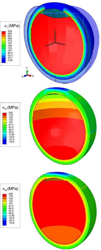
Figure 5. The radial stress  calculated using FEM with the top of the sphere shielded,
  for
for  . The deformed mesh is superimposed with the deformation scaled by 200. Parameters as in case study 1. The
  and
and  components are shown in the middle and lower figure with the same colour scale as each other.
Download figure:
Standard image High-resolution imageHalf of the spherical shell was simulated at sufficiently high resolution, requiring  elements. Unlike in the spherically symmetric cases 1 and 2 illustrated in figure 4, the shear stress
  is now non-zero. Near the interface between the shielded and unshielded regions a stress concentration of
  is clearly visible, as shown in figure 6. Away from the the shielded region the stress is very close to the the analytical solution and the symmetric FEM solution; this is as expected. This case study demonstrates that the FEM implementation of the method based on equations (49) and (50) is completely general and can be applied to any reactor geometry and boundary conditions, provided a sufficiently fine FE mesh is used.

Figure 6. The in plane shear stress component  calculated using FEM close to the interface between the shielded and unshielded region at
  , where a stress concentration is observed. Displacements are scaled by a factor of 100. The highest value of stress
  is found close to the inner surface of the shell at
  . The segment of the shell shown in this figure is a magnified part of the structure shown in figure 5.
Download figure:
Standard image High-resolution image
8. Conclusions
The treatment developed in this paper shows how to compute stresses, strains and swelling in components of a nuclear fusion or fission reactor resulting from the accumulation of defects in materials exposed to irradiation. By deriving the fundamental macroscopic equations from the atomic scale, we show that populations of radiation defects accumulating in the materials produce internal body forces (29) and (49) that result in the build-up of internal stresses and cause macroscopic deformation of components. The central notion of the treatment is the spatially varying density of relaxation volumes of defects (21), which acts as a source of stresses and strains, and the gradient of which generates the spatially distributed body force (29). We illustrate applications of the method using exact analytical solutions and numerical finite element implementations, which suggest that the method is able to provide a reasonably accurate first-principles based foundation for the in silico engineering assessment of operational performance of a fusion power plant and its design.
Acknowledgments
This work has been carried out within the framework of the EUROfusion Consortium and has received funding from the Euratom research and training programme 2014–2018 under grant agreement No 633053 and from the RCUK Energy Programme [grant number EP/P012450/1]. The views and opinions expressed herein do not necessarily reflect those of the European Commission. We gratefully acknowledge stimulating discussions with A.P. Sutton, C.H. Woo, F. Hofmann, M. Rieth, M. O'Brien and J.W. Connor. SLD is grateful to I. Lindsey and M.M.E. Coolsen who enabled this research to be carried out. ET acknowledges support from EPSRC through fellowship grant, EP/N007239/1. AES acknowledges support from the Academy of Finland through project No. 311472.