


Abstract
The interplay of flows and turbulence in Ohmic FT-2 tokamak plasmas is analysed via gyrokinetic simulations with the flux-driven ELMFIRE code. The simulation predictions agree qualitatively with analytical estimates for the scaling of the neoclassical radial electric field as a function of collisionality for ad hoc parameters. For the experimental parameters, the global full-f modeling agrees well with the analytical estimates in a neoclassical setting, while including kinetic electrons and impurities has a small impact. Allowing turbulence to develop modifies the  flow profile through relaxation of profiles caused by turbulent transport, non-adiabatic response of passing electrons around rational surfaces, and turbulent flow drive. Geodesic acoustic mode (GAM) is the main zonal flow component in the simulations, and its frequency and amplitude agree with theoretical predictions and experimental measurements. In the simulations, the non-linear energy transfer from the turbulence to the flows through the Reynolds force is balanced by the collisional flow dissipation. Temporal relationship between the oscillating flow, Reynolds force, and turbulent particle flux is consistent with the fundamental physics picture of GAM modulating turbulent transport on the time scale of the mode. Experimental evidence also suggests anti-correlation of GAM amplitude and turbulent fluctuations.
Export citation and abstract BibTeX RIS
1. Introduction
Accessing improved confinement modes (e.g. the H-mode) is required for sufficient fusion power performance in future burning plasma experiments and reactors. The physics-based understanding of transitions to e.g. H-mode has increased over the years, building on the interaction of turbulence and flows, where the latter are shaped by neoclassical physics but also driven by turbulence [1]. Axisymmetric  flows are known to suppress transport by shearing turbulent eddies, which makes the gradient of the flow a crucial parameter [2]. The standard method for estimating the effectiveness of the suppression is to compare the linear growth rate of turbulence to the average shearing rate of the flows, but if the ultimate goal is to understand the transitions to improved confinement, the model should account for the non-linear interplay of the neoclassical and turbulent components of flows and transport.
Neoclassical physics gives the base level for the  flows through the radial force balance. The well-known theory connects the mean radial electric field to plasma pressure profiles and parallel flows as presented e.g. by Hinton et al [3] and Hirshman et al [4]. The fundamental predictions of the analytical formulas have been verified by more involved simulation models [5–7], and there is experimental evidence for the neoclassical nature of the radial electric field in H-mode plasmas [8]. Global gyrokinetic modeling of ion temperature gradient (ITG) turbulence shows that accounting for neoclassical physics changes e.g. the frequency and amplitude of transport events [9].
Turbulence-driven zonal flows modify the  flow pattern set by the neoclassical physics, and they are expected to be important in confinement transitions [10–12]. Zonal flows are typically categorised into slowly evolving and finite frequency components, the latter of which is called the geodesic acoustic mode (GAM). Simulations and experiments indicate that the low frequency zonal flows shape the mean plasma pressure profiles via the shearing mechanism due to their finite radial wavenumber kr. Experiments at Tore Supra confirm the existence of staircase-like
  flow pattern and associated corrugations in the average pressure profiles as predicted by the gyrokinetic GYSELA simulations [13]. The corrugations divide the plasma into regions where avalanche-like transport events and associated bursts of flow propagate. While the GYSELA modeling utilises the adiabatic electron assumption, kinetic electron studies with the GENE, GYRO, and ORB5 codes predict that the non-adiabatic response of passing electrons has an impact on the mean profiles as well [14–16]. The simulations demonstrate that the electron diffusivity increases on flux surfaces with low order rational values of safety factor, which creates a similar staircase-like pattern that should not meander radially but remain fixed in time.
There is also evidence to indicate that the geodesic acoustic mode controls turbulent transport and influences confinement transitions, although the exact role of the mode in e.g. L-H transition is unclear [17–22]. The basic signatures of the GAM are an axisymmetric ( ) potential fluctuation, m = 1 density perturbation, finite radial wavenumber, and a finite temporal frequency [23]. It can thus impose a spatio-temporal pattern on turbulence and transport through the shearing mechanism, but the comparison of linear growth rate and shearing rate becomes non-trivial. Hahm et al [24] suggest the calculation of effective shearing rate that combines the mean and temporally varying components while discounting the impact of the latter. With this method, estimating the combined effect of GAM, low frequency zonal flows, and neoclassical background flow should be possible.
We apply the gyrokinetic simulation code ELMFIRE to study the interplay of neoclassical  flows, zonal flows, and turbulence in Ohmic plasmas at the FT-2 tokamak. The non-linear simulations with the flux-driven full-f model contain the necessary ingredients via collisions and electrostatic self-consistent turbulence. Experimental measurements have already demonstrated the anti-correlation of turbulent fluctuations and GAM activity in the discharges, while simulations predicted and experimental measurements confirmed an isotope effect on particle confinement [25, 26].
Here the simulation predictions of the radial electric field are first compared to the analytical theory for a reference case in a neoclassical setting. We then extend the analysis to the Ohmic FT-2 discharges with hydrogen and deuterium plasmas to highlight the different physics features and their impact on the mean  flow, GAM, and plasma self-organisation. Simulations demonstrate the role of rational surfaces on flows and turbulence in additional details while predicting flow values close to the experimental measurements. The simulated GAM characteristics agree with measurements and analytical predictions, and similar features are seen in turbulent particle flux. Pumping of the zonal flow is quantified via the Reynolds force and power, which are estimated to be balanced by collisonal dissipation. On the time scale of the GAM, the temporal phase relationship supports the picture of GAM modulating turbulence and so influencing turbulent transport.
2. The full-f simulation code ELMFIRE
ELMFIRE is a plasma turbulence simulation code based on gyrokinetic theory and particle-in-cell method [29, 30]. It solves the equations of motion and the gyrokinetic quasineutrality equation for the full distribution function (full-f) of electrons, main ions, and one impurity ion species. The simulations are flux-driven with the source provided by Ohmic heating and the sinks by radiation losses and the material boundary. Collisions between particles are calculated according to a momentum and energy conserving binary collision model [31]. As a consequence of the aforementioned features, the density and temperature profiles are allowed to evolve during a simulation that contains self-consistently both neoclassical and electrostatic turbulent physics. Interplay of large orbit widths, steep gradients, and different scales are included due to the global simulation geometry that covers the whole plasma volume from the axis to the wall. The circular and concentric flux surfaces of the fixed magnetic background are defined by a static input current profile, as magnetic fluctuations are excluded.
ELMFIRE simulations include both ion species as gyrokinetic, while electrons are treated drift-kinetically with the default settings. The kinetic electrons allow simulation of trapped electron mode (TEM) turbulence and non-adiabatic response of passing electrons. Their inclusion is enabled by a hybrid explicit-implicit solver that stabilizes the numerical  mode and enables longer time steps. The solver is based on an alternative definition of gyrocenter that adds an explicit polarisation drift term into the equations of motion for the ions and removes the polarisation density from the gyrokinetic quasineutrality equation

where  stands for the charge density of particle species σ and
  is the vacuum permittivity. An adiabatic electron model can also be applied in the solver as
where ni,0 is the flux-surface-averaged ion density just after initialisation of the simulation, e the elementary charge, and ϕ the electrostatic potential. To study the neoclassical physics in the following sections, we average the charge separation over the flux surfaces before solving the electric potential to remove turbulent fluctuations, i.e. modes for which  or
or  .
.
The flux-driven ELMFIRE simulations include Ohmic heating, radiation losses, and particle recycling as sources and sinks. The Ohmic heating provides a heat source for the electrons. It is applied through a loop voltage that creates a parallel electric field and accelerates the electrons. A feedback algorithm adjusts the loop voltage during the simulation to keep the plasma current consistent with the current of the static magnetic background [32]. Radiation losses are included as an energy sink for the electrons according to a pre-determined power distribution. The losses are applied at each time step and conserve the pitch angle of the particles. For  , the binary collisions provide an energy sink for electrons and a source for ions, as the collisions transfer energy from electrons to ions. Simulations conserve the total number of particles as the particles exiting the simulation domain are recycled back into it as ion-electron pairs (or groups, depending on the charge number of the ion) according to a pre-defined distribution. The magnitude of the particle source varies in time, for it depends on the number of particles crossing the material boundary. The temperature of the recycled particles is fixed to the temperature at the boundary. When applying the neoclassical averaging in the solver, the energy sources and sinks are generally disabled maintain the initial temperature profiles in the absence of turbulent transport.
A more detailed overview of the code features, including equations of motion, boundary condition implementation, and studies on energy and momentum conservation for the same plasma parameters, is presented in [33]. Previous comparisons have demonstrated ELMFIRE's ability to match experimental measurements of temporally oscillating and mean flows in the FT-2 tokamak [34, 35]. The code had also been applied to study the isotope effect on turbulent particle transport observed in experiments [25, 26].
3. Verification of neoclassical Er predictions in ELMFIRE simulations
ELMFIRE predictions of neoclassical radial electric field are compared to analytical estimates in a collisionality scan with arbitrary tokamak and plasma parameters in large aspect ratio limit (R0/a = 5) as in [6]. Comparisons have been performed with the annulus version of the code earlier [34]. Here we apply the recently developed full torus version of the code with the magnetic axis included. Plasma profiles are hyperbolic according to the formula
where X is either density or temperature and parameters X0,  , and LX control the profile shape. Temperature and density are taken equal for electrons and ions so that T0 = 368.0 eV,
  ,
,  ,
,  m−3,
m−3,  , and
, and  . These parameters produce clear maximum gradients and minimum Er in the middle of the simulation domain at r/a = 0.5, while finite orbit width effects are negligible (
 ). The safety factor profile is set to
but the plasma current is not consistent with the magnetic background due to zero loop voltage.
Plasma profiles and parameters remain constant across the different simulation cases, as collision frequency is multiplied artificially by 10, 100, and 1000 in the ELMFIRE collision subroutine to vary the collisionality. The base case is a banana regime simulation with low collisionality ( at r/a = 0.5). Simulations include no sources or sinks and only the axisymmetric radial electric field as the charge separation is flux-surface-averaged before solving the potential. Excluding turbulence and the flows driven by it allows the study of neoclassical physics and usage of a sparser grid (
![$8\times 124\times [1-150]$](https://content.cld.iop.org/journals/0029-5515/58/11/112006/revision2/nfaacf52ieqn023.gif) grid cells in toroidal, radial, and poloidal directions, respectively) compared to turbulent simulations. Adiabatic electron model and exclusion of impurities simplify the comparison and reduce the amount of computational resources needed as well. Depending on the collisionality, either the ion collision time or the ion transit time determines the time step used.
grid cells in toroidal, radial, and poloidal directions, respectively) compared to turbulent simulations. Adiabatic electron model and exclusion of impurities simplify the comparison and reduce the amount of computational resources needed as well. Depending on the collisionality, either the ion collision time or the ion transit time determines the time step used.
Hinton and Hazeltine (H–H) [3] present an analytical formula that relates the radial electric field to parallel ion flow, ion density gradient, and ion temperature gradient as
The dimensionless ion flow coefficient k is fit as a function of ion collisionality  and local inverse aspect ratio
  as
as
The ion collision frequency  is calculated as

where lnΛ is the Coulomb logarithm. The collisionality is the ratio of the collision frequency to the transit time of passing particles, i.e.
where qs is the safety factor. With this definition, the boundary between Banana and Plateau regimes lies at around  and the transition from Plateau to Pfirsch–Schlüter regime occurs at
  . For the benchmark case,
  in the middle of the simulation domain at r/a = 0.5. The Hinton–Hazeltine (H-H) fit for k converges to k = 1.17 in the Banana regime for small inverse aspect ratio. Additionally, the moment approach of Hirshman and Sigmar [4] presents another estimate for Er or k. For single ion species, their analytical expression reduces to equation (5) and k depends on the viscosity and friction coefficients. The estimates for the Hirshman–Sigmar (H–S) formula are calculated here according to the presentation of Kessel [36].
ELMFIRE predictions agree well with the analytical formulas for the scaling of mean radial electric in Banana and Plateau regimes (figure 1). The simulated radial electric field prediction is calculated from the radial derivative of the flux-surface-averaged potential  as
as
where the deviations of the potential from the flux-surface-average would anyway be negligible due to averaging of the charge separation in the solver. Meanwhile, all the quantities in equation (5) are either directly diagnosed in ELMFIRE simulations or can be calculated from e.g. the density and temperature profiles, including the toroidal rotation contribution  . This enables the calculation of the analytical predictions directly from the simulation data. The simulation results are within 15% of the Hirshman–Sigmar estimate, while ELMFIRE systematically predicts larger absolute Er values than the Hinton–Hazeltine formula in the Banana and Plateau regimes. The scaling changes qualitatively in the transition to highly collisional Pfirsch–Schlüter regime: ELMFIRE predicts the lowest absolute value but stays within 15% of the Hirshman–Sigmar model. The Pfirsch–Schlüter prediction of the simulation code is also still consistent with the scaling in the Banana and Plateau regimes. The Er values presented here effectively correspond to the ion flow coefficient k in the Hinton–Hazeltine formula, and the results are in agreement with the benchmarks of other drift-kinetic and gyrokinetic codes [5–7]. According to earlier studies [5, 37–39], the differences between the two analytical estimates are explained by the sensitive dependency of k on both
  and
and  , the latter of which is finite here (
 at r/a = 0.5) but assumed small in the Hinton–Hazeltine formulation.
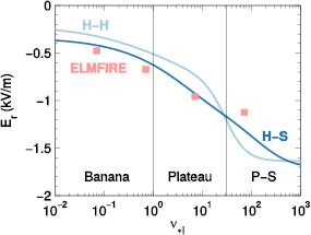
Figure 1. Radial electric field predictions by ELMFIRE and analytical theories as a function of collisionality for r/a = 0.5 in the collisionality scan. ELMFIRE predictions are based on the adiabatic electron model. The vertical lines indicate the approximate transitions between the neoclassical transport regimes.
Download figure:
Standard image High-resolution imageThe neoclassical ELMFIRE simulations converge to an equilibrium typically within a few ion collision times  , although the radial electric field retains some temporal fluctuations. For low collisionalities, the convergence happens faster in units of
  , while mean ion transit time is a better characteristic time scale for the high collisionalities. Including kinetic electrons does not change the convergence behaviour of Er in the plateau case, even though the time step needs to be decreased to account for the fast parallel movement of the electrons and the computational effort is increased by an order of magnitude. The equilibrium values for kinetic and adiabatic electrons are on average within 5% of each other and the Hirshman–Sigmar prediction (figure 2) for the plateau case. The limited impact of kinetic electrons is expected based on the kinetic studies of Belli et al [5], but it could become meaningful in situations where electron and ion temperature profiles are drastically different.
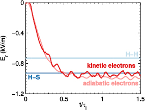
Figure 2. The convergence of the radial electric field in ELMFIRE simulations with adiabatic and kinetic electrons compared to the analytical predictions. The ion collision time is  μs in this plateau regime case. Some temporal Er fluctuations remain for both kinetic and adiabatic electrons.
Download figure:
Standard image High-resolution image4. Non-linear simulations of FT-2 tokamak plasmas
4.1. Discharges and simulation setup
Experiments have been conducted for similar hydrogen and deuterium discharges in the low current regime at the FT-2 tokamak ( kA,
kA,  T) [25, 26]. The large aspect ratio tokamak (R0 = 55 cm, a = 7.9 cm) has a circular cross section and a limiter configuration. The plasmas studied here have similar temperature and density profiles (Ti = 150 eV, Te = 440 eV, and
  m−3 at axis as seen in figure 3), while impurity fraction is larger for deuterium (
 ) than for hydrogen (
 ). Spectroscopic measurements and temperature profiles point to partially ionised oxygen O6+ being the main impurity. The radial
  profile is assumed to be uniform. High collisionality and large ion orbit widths (
 and
and  cm) characterise the parameter regime of the FT-2 plasmas. More detailed description of the discharges is available in [25, 26].

Figure 3. Input, error estimate, and ELMFIRE predictions of the density and temperature profiles for the hydrogen case. The ELMFIRE prediction has been averaged over the turbulent phase of the simulation (150 μs).
Download figure:
Standard image High-resolution imageExperimental measurements have found anti-correlation between the turbulence level and GAM activity in the discharges [25]. The simultaneous measurements of plasma poloidal velocity oscillations associated with the GAM and turbulent density fluctuations were performed using a combination of Doppler enhanced scattering (ES) and standard equatorial probing O-mode reflectometry. ES is a microwave technique that utilises the backscattering off the small scale density fluctuations in the probing wave upper hybrid resonance [27, 28]. The diagnostics also provide mean  flow measurements. The discharges were divided into time periods of strong and weak GAM amplitude, and the comparison of turbulent spectra between these periods shows that the turbulent fluctuations decrease when GAM amplitude is larger. This indicates that the the flow oscillations are able to suppress the turbulence. The effect is stronger for the deuterium discharge compared to hydrogen. At the same time, particle source estimations based on the Hβ and Dβ line radiation measurements indicate an isotope effect on particle confinement for the discharges [26].
We apply the gyrokinetic code ELMFIRE to study the interplay of flows and turbulence in these discharges. The simulation grid allows the resolution of turbulence for  inside r/a = 0.63, after which resolution declines to
  at r/a = 1.0. Unlike in [25], the computations now cover the plasma from magnetic axis to the wall and both poloidal and radial resolution vary radially. A total of
  (
( ) grid points and
  (
( ) particle markers are used to obtain grid size equal to ion Larmor radius
  in radial and poloidal direction up to r/a = 0.63 and an average of 7400 (7800) markers per grid cell in the hydrogen (deuterium) case. The particle count is sufficient to keep the noise below 1%, while no noise accumulation occurs in full-f simulations [34]. The time step is
  ns in this case, and it is mainly limited by the accuracy condition for the parallel electron streaming, i.e.
  , and the number of toroidal grid cells (Nz = 8 in this case) [40].
Available computational resources and the balance between sources and sinks limit the total physical time of these flux-driven simulations, which is relatively short (180 μs  ). The energy confinement time of the discharges is approximately
  ms, and the particle confinement time is understood to be longer. As a perfect match between sources and sinks is not achieved, the mean profiles slowly diverge from the experimental equilibrium that is used as an input. The effect is worse for the hydrogen parameters (figure 3). The deviation is within error bars for density and ion temperature, but the electron temperature relaxes strongly at the edge. The total energy of the plasma increases with a rate of 18.3 kW in the end of the hydrogen discharge simulation compared to the estimated Ohmic input power of 48.5 kW. The total particle number remains constant due to the source model employed by ELMFIRE but the preset recycling profile does not completely match the flux profile, and so the density profile relaxes mainly by accumulating ions and electrons at the edge. As the particle confinement time is longer than the energy confinement time, the density profiles are maintained closer to the input during the simulation.
4.2. Mean  flow characteristics

ELMFIRE predictions agree better with the Hinton–Hazeltine analytical formula than with the Hirshman–Sigmar estimate for FT-2 parameters when turbulence is excluded from the calculations (figure 4). For this comparison, only the flux-surface-averaged charge separation is again solved (m = 0, n = 0) and three different physics settings are applied to simulations of the hydrogen discharge: adiabatic electrons, kinetic electrons, and kinetic electrons with impurities (O6+). The collisionality of the plasmas lies in the transition zone between Plateau and Pfirsch–Schlüter regimes depending on the radial position ( ). The good agreement with the Hinton–Hazeltine formula is in contradiction with the collisionality scan presented earlier. Finite orbit width (FOW) effects are the most likely explanation for this change, because inverse aspect ratio values are similar to the parameters used in the collisionality scan and cannot thus explain the difference. The analytical predictions agree on the very edge as the plasma transitions completely to the Pfirsch–Schlüter regime.

Figure 4. Time averaged Er profile predicted by ELMFIRE with different physics settings (adiabatic electrons, kinetic electrons, and kinetic electrons and impurities) for the neoclassical hydrogen case and the analytical formulas from Hinton–Hazeltine and Hirshman–Sigmar. The analytical predictions are calculated according to the profiles of the kinetic electron case and as such they include orbit loss effects.
Download figure:
Standard image High-resolution imageAgreement between ELMFIRE results and the Hinton–Hazeltine formula is very good in the core, where the plasma is more in the plateau regime. Towards the edge the agreement worsens as the plasma transits to the collisional regime and the temperature gradient term starts to have a larger influence on the total Er (figure 5). This is to be expected based on the collisionality scan. Toroidal rotation has a negligible effect on the radial electric field for these parameters: it is largest at 0.7 < r/a < 0.8, where it corresponds to 6.5% of the total Hinton–Hazeltine analytical prediction in the hydrogen case and on average to just 3.0%. Inclusion of kinetic electrons also changes the behaviour of the boundary condition and introduces a clear orbit loss effect that results in a wide radial electric field well on the edge. The analytical formula captures a part of the orbit loss effect as the inclusion of kinetic electrons causes a depletion of density and temperature very close to the wall. Otherwise the effect of kinetic electrons and even impurities is small despite the finite effective charge values ( in the hydrogen case of figure 4). The former result is in agreement with results from the collisionality scan.

Figure 5. Time averaged Er profile in the hydrogen case as predicted by the analytical Hinton–Hazeltine formula and a neoclassical ELMFIRE simulation with kinetic electrons and without impurities. The coloured lines without markers indicate the three different terms in equation (5).
Download figure:
Standard image High-resolution imageInclusion of turbulence significantly alters the Er and thus the  flow and shear profiles in ELMFIRE simulations (figures 6 and 8). This is caused by three main factors: pressure profile modifications due to transport of energy and particles, turbulence-driven flows (low frequency zonal flows and finite frequency geodesic acoustic mode), and the non-adiabatic response of passing electrons. The first factor is clearly seen by comparing the analytical prediction for the initial profiles and the profiles averaged over time. Heating of the plasma reduces temperature gradients and ion collisionality in r/a = 0.6–1.0, which decrease the
  contribution to Er in the analytical formula. The parallel flow term
  in equation (5) increases to 6.1% of the total Er prediction on average from the 3.0% in the neoclassical simulations. The prominent Er well seen in the neoclassical simulations narrows down, as the turbulent particle flux dominates over the orbit loss mechanism near the boundary.
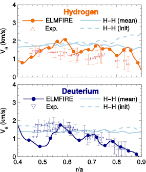
Figure 6. The mean  flow in the turbulent phase of simulations as predicted by ELMFIRE, Hinton–Hazeltine analytical formula, and the experimental measurements of poloidal flow. The data is shown for the measured radial interval. Mean values for analytical and simulation predictions have been averaged over 30 μs in the saturation phase of the simulation to minimise the effect of profile relaxation.
Download figure:
Standard image High-resolution imageTurbulence-driven zonal flows are the main reason for the deviation of ELMFIRE prediction from the analytical Hinton–Hazeltine estimate. This is seen by comparing the difference in the mean  flow predictions and the turbulent flow drive (figure 7). Unlike in the comparison to the experimental measurements in figure 6, there is no need to consider how close the plasma profiles are to the input in this case, so the values are averaged over the whole saturated phase of the simulation lasting 150 μs. The simulated
  flow
flow  is again calculated directly from the flux-surface-averaged radial electric field as
  , while the Er prediction of equation (5) is used for
  based on the Ti, ni, and
  profiles from the same simulation and time interval. The turbulent drive is quantified by Reynolds stress

and its derivative, the Reynolds force


Figure 7. The difference between poloidal  flow
flow  predicted by ELMFIRE and Hinton–Hazeltine analytical formula compared to the average radial distribution of the Reynolds force in the hydrogen case. Ion diamagnetic direction is in the positive direction. Both the velocity difference and the Reynolds force are averaged over 150 μs in the saturated phase.
Download figure:
Standard image High-resolution imageHere  and
and  are taken as the radial and poloidal
  drifts, respectively, while
  denotes averaging over the flux surface. The time averaged Reynolds force correlates strongly spatially with the deviation of the simulated
  flow from the analytical values. Additionally, there is a significant temporally varying Er component due to the geodesic acoustic mode, which is discussed in the following subsections.
The sharp zig-zag-like pattern of the flow and its shear is associated with the rational surfaces and the non-adiabatic response of passing electrons at these surfaces (figure 8) [15, 16]. The often used adiabatic electron assumption breaks down around surfaces for which the safety factor has values qs = −m/n, where m and n are small integers. The parallel wavenumber vanishes as  and the adiabatic condition
  is violated at and around the surface. As a consequence, the passing electrons also participate in turbulent fluctuations, which increases electron temperature fluctuations and electron diffusivity around rational surfaces. Electron temperature and density thus flatten at e.g. qs = 2.0 and steepen around it to account for the pattern in diffusivity. The impact on the ion temperature profile is limited, as observed earlier by Waltz et al [14]. The flow shear is close to zero at the rational surface and minimum and maximum next to it where the pressure profiles are steepened. The shear pattern stays fixed at these magnetic surfaces unlike the meandering
  staircase observed by Dif-Pradalier et al [13]. Comparison of simulation and analytical predictions indicates that the fine structures are larger in amplitude than the neoclassical theory would predict based on the morphing of the profiles (figure 7).
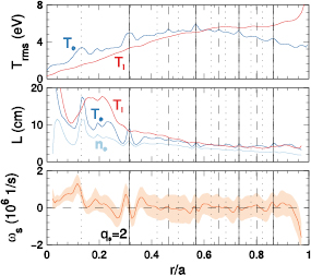
Figure 8. In ELMFIRE simulations, the non-adiabatic response induces larger electron fluctuations at flux surfaces with rational safety factor qs values. These surfaces are indicated by vertical lines here: solid lines for integer surfaces, dashed for half integer surfaces, and dotted for 1/3 surfaces. Top figure: the root mean square values ( ) of Te fluctuations increase at rational magnetic surfaces, while ion fluctuations are largely uninfluenced. Middle figure: this also impacts the mean Te and ne profile steepness, but influence on Ti profile is negligible except very close to the axis. Bottom figure: the corrugations in the mean flow shear
  are visible for mostly integer values of qs. The shaded area indicates the standard deviation of
  .
.
Download figure:
Standard image High-resolution imageThe parameter range and model employed in this manuscript have some crucial differences relative to the other work where similar flow patters have been identified. The interplay of rational modes and radial electric field is complicated by neoclassical background, full-f model, impurities, collisions, and flux-driven nature of the simulations compared to the work of Dominski et al [15, 16], while inclusion of impurities and kinetic electrons were missing in the studies of Dif-Pradalier et al [13]. The inclusion of kinetic electrons is crucial for the development of the staircase-like pattern presented in this manuscript and work of Dominski et al, as it enables the simulation of resonant modes, the effect of which could be exacerbated by the the temperature ratio  . Meanwhile, impurities effectively change the collisionality of the plasma and influence the neoclassical radial electric field profile, increase the damping of zonal flows, and inhibit the linear growth of turbulence. The local flattening of the profiles, changes in Er and turbulent fluctuation profiles, and localisation on rational modes have similarities with magnetic islands associated with internal transport barriers (ITBs) [41], although as an electrostatic code ELMFIRE cannot simulate their formation. Waltz et al also note that the effect of rational surfaces was observed with electrostatic simulations and without the magnetic signature of islands in experiments. Due to the short simulation time, the spatio-temporal flow pattern of the geodesic acoustic mode also plays a role in defining the averaged flow profile as it propagates radially and its amplitude evolves in time.
The  flow
flow  predictions by ELMFIRE agree well with experimental measurements of poloidal flow on average in both discharges (figure 6). The experimental values are based on the Enhanced Scattering diagnostic which measures the velocity of plasma fluctuations as a sum of the
  drift and the phase velocity of the fluctuations
  . In the comparison of figure 6, the term
  is effectively neglected by taking
  . The phase velocity contribution is generally smaller than the uncertainty of the measurements based on local linear gyrokinetic simulations with GENE [42]. As the measurements pick the phase velocity for known wavenumbers at each radial position, the contribution of the phase velocity to the measurements can be estimated via the linear gyrokinetic simulations. For r/a = 0.63 in the hydrogen case, the
  value is based on poloidal wavenumber
  and the simulations predict
  m s−1 in the ion diamagnetic direction. Collisions and impurities are included in these linear calculations.
The small-scale corrugations of the flow pattern cannot be compared to experiments due to limited resolution of the measurements, but the differences between the analytical Hinton–Hazeltine predictions and measurements indicate that either there are significant turbulent contributions or that the actual plasma profiles deviate meaningfully from the ones used in the simulations and ASTRA analysis, or a mix of both effects. Given the uncertainty in the ion temperature and that the  values based on the relaxed profiles are closer to the measurements, the ion temperature profile may be actually less steep at the edge than is used as an input for simulations. Uncertainties in e.g. impurity distribution and safety factor profiles and their impact on the
  flows are more difficult to quantify and would require more extensive and specific studies.
4.3. Oscillating flow characteristics

The oscillating component of the flow exhibits the basic characteristics of the geodesic acoustic mode with axisymmetric (m = 0, n = 0)  poloidal rotation and the associated m = 1 up-down asymmetric density fluctuation. The dominating frequency of the flow oscillations is within 20% of experimentally measured values and theoretical prediction for the geodesic acoustic mode frequency (figure 9). The radial slope of the frequency profile in experiments and simulations is consistent with continuum-type GAM, for which the frequency of the mode scales according to the local plasma properties. Considering the density and safety factor profiles of the discharges, this is in line with computational and experimental evidence from TCV [44, 45].

Figure 9. Top: the colormap represents the poloidal  flow power spectrum predicted by ELMFIRE for the hydrogen parameters. The values are normalised to the peak amplitude for each radial coordinate. The dark regions correspond the peak amplitude. They coincide with theoretical prediction (lines) and experimental measurements (markers) for GAM frequency. Solid lines indicate analytical estimate for initial profiles, while dashed line uses the mean profiles in the saturation phase. Bottom: GAM amplitude based on the Fourier component (solid line) at
  and the standard deviation of
  in ELMFIRE simulations compared to the experimental GAM amplitude distribution (markers).
Download figure:
Standard image High-resolution imageThe theoretical prediction of the GAM frequency has been calculated according to the dispersion relation derived by Guo et al [43], which accounts for impurities and finite orbit width effects. The O6+ impurities are included according to ELMFIRE density profiles that are consistent with the experimental effective charge  in the beginning of the simulation, while experimental value is used for the radial wavenumber kr, for the experimental measurements and computational predictions of
  have previously been shown to be close to each other [28]. For the hydrogen case, the simulations predict
  cm and measurements indicate
  cm, which agree within uncertainties. Relaxation of the temperature and density profiles is a characteristic feature of the flux-driven full-f simulations. In this case it mainly increases temperatures and thus expected frequencies in the edge plasma, and accounting for the relaxation improves the agreement between the analytical estimate and ELMFIRE prediction.
The amplitude of the oscillating flows is large enough to momentarily even reverse the poloidal  rotation from electron diamagnetic to ion diamagnetic direction in experiments and simulations (figure 9). This is in agreement with L-mode experiments in other tokamaks [19, 46, 47]. Comparison of Fourier analysis and standard deviation of the Er time series shows that the latter is a good substitute for the GAM amplitude in ELMFIRE simulations of FT-2 plasmas due to the prominence of the oscillating mode. In fact, the standard deviation provides a better match for the experimental values. For the radial electric field, it is approximately 4.0 kV m−1 at r/a = 0.5 in both cases, while the mean value is
  kV m−1. As a consequence, the oscillating component of flow shear rate dominates over mean flow shear in most of the plasma volume (figure 8). The peak GAM amplitude is larger by a factor of two in the deuterium case compared to hydrogen, although the difference in the maximum standard deviations of
  is only approximately 50% as in the experiments. Given the propagation of the GAM in radial direction, longer simulations with improved power balance and reduced profile relaxation could improve the agreement between simulations and experiments.
4.4. Interaction of GAM and turbulence
The geodesic acoustic mode is excited in the non-linear saturation phase of the simulations, and the frequency and propagation signature of the GAM are also visible in other quantities as avalanche-like bursts that propagate mostly inwards in radial direction. This is a manifestation of the non-linear coupling of turbulence and flows. Turbulence transfers part of its energy to the flow, which is then dissipated by the damping of the flow back into the bulk plasma. In the following, we analyse this interaction in ELMFIRE simulations. We use the frequency associated with the peak Er component predicted by ELMFIRE as the characteristic GAM frequency  . This definition breaks down close to the axis, where the GAM signatures disappear.
The linear growth rate of the trapped electron mode (TEM, driven by the density gradient in these discharges) turbulence is approximately  s−1 at r/a = 0.63 in both discharges [26]. The standard deviation of the shearing rate
  easily exceeds this, while the mean value does not. It is difficult to draw conclusions by comparing the mean flow shear directly to linear growth rates, because also the mean electron temperature and density profiles steepen around the rationals in flux-driven full-f simulations as discussed earlier. The linear analysis is conducted with the initial profiles and the local morphing of profiles by transport is not taken into account.
The combined effect of mean and oscillating shear can be strong enough to provide significant rotation shear for turbulence suppression once or twice per GAM period. According to the theory proposed by Hahm et al [21, 24, 25], a condition for the effective shearing rate can be written as

where  is the mean and
  the fluctuating component of the shearing rate
The reduction factor ![$H\, =\, \left[\left(1\,+\,3F\right){}^2\,+\,4F^3\right]^{1/4}\,/$](https://content.cld.iop.org/journals/0029-5515/58/11/112006/revision2/nfaacf52ieqn122.gif)
![$\left[(1+F)\sqrt{1+4F}\right]$](https://content.cld.iop.org/journals/0029-5515/58/11/112006/revision2/nfaacf52ieqn123.gif) (with
(with  ) discounts the effect of the oscillating flow shear, since it is not as effective in suppressing turbulence as a stationary shear. The suppression mechanism itself is not sensitive to the sign of the gradient, but
  is on average large enough to guarantee that the condition in equation (12) is fulfilled only in one half of a GAM period, i.e. when the mean and fluctuating component have the same sign.
The effective shearing manifests itself as a modulation of particle flux at the GAM frequency, and the effect is stronger in deuterium due to larger effective shearing rate. The spatial average of absolute mean shearing rate is  kHz (105 kHz) in r/a = 0.4–0.9 of the hydrogen (deuterium) case, while the standard deviation is
  kHz (717 kHz) and reduction factor H = 0.56 (0.60) in the same interval. The clear difference in the GAM amplitude is diluted in terms of shearing rate due to larger wavelength
  of the heavier isotope since
  . Temporal phase shift between the flow shear and particle flux is close to
  at the GAM frequency in both cases (figure 10). The flow shear follows the particle flux, and this relationship holds for the wide radial range where the GAM exists. The phase shift α is calculated as a function of temporal frequency f as
 ![$\alpha(\,f) = \mathrm{arg}[\omega_s^\ast(\,f) \Gamma_e(\,f)]$](https://content.cld.iop.org/journals/0029-5515/58/11/112006/revision2/nfaacf52ieqn131.gif) after applying a temporal Fourier transform on the flow shear
after applying a temporal Fourier transform on the flow shear  and the particle flux
  . Here * denotes the complex conjugate.
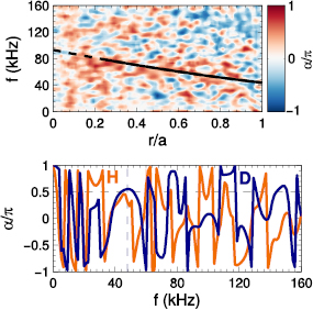
Figure 10. Top: cross-phase between poloidal  flow shear
  and electron particle flux
  (colormap) shows that they fluctuate with a phase shift close to
  at the GAM frequency (solid line) in the hydrogen case. Bottom: one-dimensional cross-phase distribution at r/a = 0.63 for hydrogen (orange, larger
  ) and deuterium (dark blue, smaller
  ) shows that the phase shift is consistent for both isotopes. The vertical dashed lines correspond to
  .
.
Download figure:
Standard image High-resolution imageAs in the case of the mean flow, we quantify the turbulent flow drive via Reynolds stress  and its derivative Reynolds force
  . The Reynolds power density or the energy transfer from the turbulence to the flow per unit of time in unit volume is calculated as

where  stands for the poloidal
  rotation based on the axisymmetric radial electric field in the simulations [48]. The dissipation of the GAM, meanwhile, is generally expected to be induced by collisionless and collisional damping. We focus on the latter mechanism due to high collisionality of the FT-2 plasmas (
 in the whole plasma volume for both discharges). The Landau-like collisionless damping has its maximum in the the core region because it decreases quickly with the safety factor, although finite orbit effects tend to strengthen its effectiveness [49]. Collisional dissipation depends on the ion collision frequency
  and should thus be especially significant in the edge plasma [50]. We use the basic expression
for the collisional damping with  calculated according to equation (7). To account for the effect of impurities, we multiply
  with the effective charge
  [51]. The dissipation rate of the flow energy density is then calculated as

The total Reynolds power density is approximately equal in the hydrogen and deuterium plasmas (figure 11). Balance between the Reynolds power density and collisional dissipation of equations (14) and (16) is well maintained for deuterium, except on the very edge. A more notable gap between the two remains for hydrogen parameters. This is likely due to the crude collisional damping estimate and short simulation duration. For the comparison, we have integrated the driving and dissipating power over the volume inside the magnetic surface and averaged over time. The results suggest that the drive and dissipation of the geodesic acoustic mode can be explained within the framework of Reynolds force and collisional damping in the FT-2 plasmas. This would thus support the earlier conclusion that the higher GAM amplitude in the deuterium discharge would be due to decreased collisional damping for the heavier isotope [25].
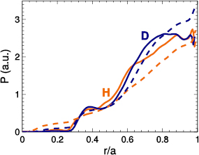
Figure 11. Collisional flow dissipation (dashed lines) is estimated to roughly balance the Reynolds power (solid lines) in the simulations. The values here have been integrated over the volume and averaged over time.
Download figure:
Standard image High-resolution imageThe Reynolds force FR alternates its direction between electron and ion diamagnetic directions by oscillating in time in the region of largest GAM amplitude (r/a = 0.4–0.8). In this radial interval, the mean value of the force is close to zero compared to the fluctuating components, while inside r/a = 0.4 the mean component starts to be significant (figure 12). The total Reynolds force fluctuations are 45% larger in hydrogen compared to deuterium according to the temporal standard deviation. As the standard deviation of the Reynolds force follows roughly the radial distribution of radial  drift fluctuation amplitude, the difference between the isotopes is largely explained by the larger turbulent
  fluctuations
  in the hydrogen case. Combining this with the equivalent Reynolds power density PR, the estimated turbulence consumption rate
  (the ratio of Reynolds power density and turbulent
  energy) is actually larger for deuterium by roughly 45%. This is not obvious when comparing just the density fluctuation levels, which are comparable for the two cases. How
  translates into
  depends on the poloidal spectra of the density and, by extension, potential fluctuations. The conclusion is nevertheless in agreement with the earlier effective shearing rate calculations.

Figure 12. Top: standard deviation (solid lines) of the Reynolds force is larger than the mean absolute value (dashed lines) in the GAM dominated region. Bottom: radial  drift fluctuations, averaged over flux surfaces and time, are larger in hydrogen and spatially correlated with the amplitude of Reynolds force fluctuations in both cases.
Download figure:
Standard image High-resolution imageThe Reynolds power density is comparable between the isotopes due to larger amplitude of the GAM and the stronger correlation between the Reynolds force and the flow oscillations in the deuterium case (figure 13), despite the difference in the Reynolds force amplitudes (figure 12). The GAM frequency dominates the temporal correlation function for deuterium in the GAM populated radial zone, while higher frequency components are clearly present in the hydrogen case. The correlation between Reynolds force and poloidal  velocity at GAM frequency becomes negligible outside the GAM dominated region inside r/a < 0.4 in the deuterium case. The phase shift
 ![$\alpha(\,f) = \mathrm{arg}[V_\theta^\ast(\,f) F_{\rm R}(\,f)]$](https://content.cld.iop.org/journals/0029-5515/58/11/112006/revision2/nfaacf52ieqn161.gif) between the Reynolds force and the flow oscillation changes sign close to
between the Reynolds force and the flow oscillation changes sign close to  , indicating a small or vanishing phase shift for that frequency (figure 14). The behavior is consistent for both hydrogen and deuterium discharges in the radial range where the flow oscillations are observable in the simulations. The energy transfer from turbulence to the flows thus depends on the spatio-temporal relationship between Reynolds force and flow in addition to their absolute magnitudes according to Reynolds power density in equation (14). The synchronised oscillations allow the positive transfer of energy from turbulence to flows.

Figure 13. Top: temporal correlation between Reynolds force (FR) and poloidal  flow is stronger in the GAM dominated zone in the deuterium simulation. Bottom: comparison between the cases is shown in the bottom graph for r/a = 0.63. The correlation functions have been normalised for each radius so that the autocorrelation functions become unity at zero timelag
  .
.
Download figure:
Standard image High-resolution image
Figure 14. Top: cross-phase between poloidal  rotation and Reynolds force (colormap) shows that they oscillate in phase at the GAM frequency (solid line) in the hydrogen case. Bottom: one dimensional cross-phase distribution at r/a = 0.63 for hydrogen (orange, larger
  ) and deuterium (dark blue, smaller
  ) shows that the phase difference is consistently small for both isotopes. The vertical dashed lines correspond to
  .
.
Download figure:
Standard image High-resolution image
5. Summary and discussion
The verification of neoclassical radial electic field predictions of the electrostatic gyrokinetic simulation code ELMFIRE was presented. A collisionality scan for ad hoc parameters without impurities found qualitative agreement with the scaling predicted by Hinton–Hazeltine [3] and Hirshman–Sigmar [4] models. The simulation predictions followed more closely the scaling given by the Hirshman–Sigmar approach in agreement with other similar benchmarks [5–7, 38, 39].
Secondly, ELMFIRE has been applied to study the interaction of  flows and turbulence in hydrogen and deuterium plasmas at the FT-2 tokamak. The discharges are characterised by Ohmic heating and thus a lack of external momentum injection. Ion collisionality lies in the Plateau and Pfirsch–Schlüter regimes, while ion orbit widths are large relative to the machine size and gradient scale lengths. The dominant trapped electron mode turbulence is driven by the density gradients, and it provides a source for substantial geodesic acoustic mode oscillations, which are favored also by the large safety factor values at the edge due to the modest plasma current.
The gyrokinetic predictions of the mean  flow agree well with the analytical neoclassical estimates. Comparison with the analytical benchmark indicates that finite orbit width effects play a role in determining the neoclassical
  flow profile in the FT-2 discharges, as the simulation predictions follow more closely the Hinton–Hazeltine prediction unlike in the collisionality scan. In the simulations, the TEM turbulence shapes the flow profile due to turbulent flow drive, non-adiabatic response of passing particles around rational surfaces, and relaxation of profiles caused by mismatch of sources and sinks. The strongest mean shear emerges around the rational surfaces, resulting in a staircase-like pattern similar to that observed in other work with kinetic electrons [14–16] but unlike the so-called meandering
  staircase [13]. Due to the electrostatic nature of the simulations, the impact of resonant modes is not associated with magnetic islands. Comparison of experimental measurements and the predictions of simulations and analytical theory supports the role of turbulence in determining the
  flow profile, but the existence of the staircase cannot be verified.
The simulations also predict strong geodesic acoustic mode activity for the discharges. The frequency and the amplitude of the  flow oscillations agree well with analytical theory and experiments. The oscillating flow matches or even exceeds the mean flow outside the very core of the plasma. It thus reverses the direction of poloidal rotation when the GAM reaches its maximum amplitude and has a strong impact on the
  shear. The spatio-temporal GAM signature is seen in the turbulent particle flux as well. Analysis of the interaction between the
  flow and the turbulence supports the conclusion that turbulence drives the flows non-linearly via the Reynolds force. The pumping by turbulence is found to be balanced by collisional damping. The driving force, the flow, and the particle flux oscillate close to in-phase in time, while the flow shear induced by the GAM follows with a phase shift of
  . The pumping of the geodesic acoustic mode by the turbulence is consistent with experiments at the FT-2 tokamak, where measurements have observed anti-correlation of turbulent fluctuations and GAM amplitude. The presence of background shear ensures that the GAM meets the criterion for suppressing turbulence only in one half of a GAM period.
The framework of collisional dissipation and turbulent drive has tentatively been applied to simulations of high current ( kA) FT-2 plasmas and both L-mode and H-mode plasmas at the TUMAN-3M tokamak [52]. The results are consistent with the work presented here. Strikingly, the TUMAN-3M H-mode simulations do not have the geodesic acoustic mode, and accordingly the Reynolds power density is negligible compared to the GAM occupied L-mode. The localisation of the profile corrugations and amplified electron temperature fluctuations also shift with the modified safety factor profile.
The imbalance of sources and sinks, especially at the edge, prevents longer simulations of the Ohmic FT-2 discharges. As the particle confinement time is estimated to be longer than the energy confinement time, the density profiles are maintained better than the temperature profiles during these short simulations, so the problem is worse for power balance. Consequently, the computations presented here are too short to analyse the energy transfer between turbulence and flows over several bursts of the GAM that are seen in experiments. They offer a glimpse into the dynamics during a single burst of flow oscillations. Further investigations into the predator-prey-like dynamics of larger time scales of typical limit cycle oscillations require better matching or adopting a different approach for the sources and sinks in addition to increased computational resources.
Acknowledgments
This work has been carried out within the framework of the EUROfusion Consortium and has received funding from the European Union's Horizon 2020 research and innovation programme under grant agreement number 633053. The views and opinions expressed herein do not necessarily reflect those of the European Commission. The work is supported by grant 278487 of the Academy of Finland. Co-authors of the paper (A. Altukhov, L. Esipov, A. Gurchenko, E. Gusakov) would like to acknowledge financial support of Russian Science Foundation grant 17-12-01110 and of the Ioffe institute. Computational resources for the work were provided by CSC—IT Center for Science and IFERC-CSC.