


Abstract
For the first time, over five confinement times, the self-consistent flux driven time evolution of heat, momentum transport and particle fluxes of electrons and multiple ions including Tungsten (W) is modeled within the integrated modeling platform JETTO (Romanelli et al 2014 Plasma Fusion Res. 9 1–4), using first principle-based codes: namely, QuaLiKiz (Bourdelle et al 2016 Plasma Phys. Control. Fusion 58 014036) for turbulent transport and NEO (Belli and Candy 2008 Plasma Phys. Control. Fusion 50 95010) for neoclassical transport. For a JET-ILW pulse, the evolution of measured temperatures, rotation and density profiles are successfully predicted and the observed W central core accumulation is obtained. The poloidal asymmetries of the W density modifying its neoclassical and turbulent transport are accounted for. Actuators of the W core accumulation are studied: removing the central particle source annihilates the central W accumulation whereas the suppression of the torque reduces significantly the W central accumulation. Finally, the presence of W slightly reduces main ion heat turbulent transport through complex nonlinear interplays involving radiation, effective charge impact on ITG and collisionality.
Export citation and abstract BibTeX RIS
1. Introduction
High-Z metallic materials, such as Tungsten (W), are chosen for their high melting point, low erosion rate and low hydrogen retention. W will be used in ITER on the divertor tiles [1]. But due to its large charge number 74, W ions are not fully ionized even in the hot tokamak core, leading to an significant level of line radiation. This means that W central core accumulation in the plasma core can be highly deleterious. To avoid central W accumulation, an accurate understanding of W transport is a key issue. In the central region of JET core, W transport has been shown to be mostly caused by neoclassical convection [2–7], whereas, in the outer part, the turbulent diffusion dominates. Neoclassical transport depends on main ion temperature and density gradients, as well as on plasma rotation. Therefore, in order to understand the mechanisms of W transport, it is crucial to predict accurately and self-consistently the time evolution of the temperature, density and rotation profiles. To do so, one needs to model the interplay between heat, angular momentum and particle, accounting for sources, losses and transport (both neoclassical and turbulent), over multiple confinement times while self-consistently modelling the current diffusion. Therefore the use of an integrated modeling tool such as JETTO [8] is mandatory.
The goal of this work is to reproduce the experimental behavior of an extensively studied JET-ILW hybrid H mode (#82722) over 5 confinement times, i.e. 1.7 s. While it has been demonstrated that MHD phenomena impact the W behavior in the core through sawteeth [9] and at the edge through Edge Localized Modes [10], they are not modeled in our simulations. This decision is based on the results of [6, 7], where, at given times, using the measured plasma background profiles, the W turbulent transport modeled by GKW [11] and the W neoclassical transport modeled by NEO [12, 13] successfully reproduce the 2D W density profile. Although, it is to note that, in these previous works, the background profiles were taken from measurements and not predicted, whereas in the present approach they are predicted self-consistently. Therefore, in our JETTO integrated modelling, the neoclassical transport is modelled using NEO and the turbulent transport using QuaLiKiz [14–16]. Due its too expensive CPU cost, GKW even in its quasilinear version cannot be integrated in JETTO, therefore QuaLiKiz is used instead. QuaLiKiz is a quasilinear gyrokinetic code which has been widely validated against other quasilinear and nonlinear gyrokinetic codes [15]. The initial W content was adjusted to match the initial bolometry signal. The W boundary condition at the Last Closed Flux Surface (LCFS) was a constant incoming fluence. The transport in the pedestal was fixed during the simulation with adjusted transport coefficients matching ELM-averaged electron density and temperature measurements. With these settings, the JETTO-NEO-QuaLiKiz modelling of the JET-ILW pulse #82722 over 5 confinement times, i.e. 1.7 s, reproduced successfully and simultaneously the electron and ion temperatures, the electron density and the toroidal rotation profiles. The modelled 2D W profiles exhibit a core W accumulation, similar, although not identical, to one observed experimentally.
Thanks to this multi-channel, multi confinement times, flux driven simulation, the W central core accumulation actuators could be identified. The W core accumulation was completely mitigated by removing the central NBI particle source. Removing the NBI torque allowed to reduce significantly the W accumulation. Showing that tokamaks with lower core fuelling and lower torque input should be less prone to core W accumulation. This was actually demonstrated experimentally on Alcator C-Mod [9] and is favourable for WEST or ITER operation. Finally, the W presence was shown to lead to an improved heat confinement through complex non-linear interplays invoking modified  due to modified radiation losses, modified effective charge and collisionality, all impacting the turbulent transport.
In section 2, the studied JET-ILW pulse is presented. In section 3, the JETTO-NEO-QuaLiKiz configuration used in this work is reviewed. In section 4, the predicted profiles by JETTO-NEO-QuaLiKiz are compared to the measured ones. Section 5 focuses on two actuators leading to W central accumulation: NBI central particle source and NBI torque. Section 6 explains the mechanisms at play behind the W stabilization effect. Finally, conclusions are drawn in section 7
2. JET-ILW plasma profiles and W core accumulation phenomenon
Understanding and modeling the mechanisms leading to central W central core accumulation (inside  ) is a key issue. In this perspective, Angioni et al [6] presents a detailed analysis of the hybrid JET-ILW shot #82722, at two time slices.
Time traces of the chosen JET-ILW pulse (#82722 BT = 2 T IP = 1.7 MA) are shown on figure 1. The time window modelled by JETTO corresponds to the shaded area, from 5.5 s to 7.1 s. In this time window, neutral beam injection (NBI) at 16 MW is the only auxiliary heating. The presence of ELMs in the pedestal is visible on the total radiated power on figure 1(a). The SXR central line t19 on figure 1(d) shows strong peakings when compared with the peripheral SXR line t22, which indicates the W central accumulation, visible also on figure 3. Around 5 s, the electron density shown on figure 1(b) has a hollow profile, which is more visible on figure 2(a). Then the central density peaks, though limited by three sawtooth crashes at 5.9 s, 6.5 s and 7.1 s, with an inversion radius at  , where ρ is the square root of the normalized toroidal flux. The sawteeth can also be seen on the central temperature on figure 1(c) and for, the one at 7.1 s, on the central SXR line on figure 1(d). The central electron temperature on figure 1(c) first increases until 5.5 s, then tends to decrease with time. Note that there is no SXR peak corresponding to the time between the sawteeth at 5.9 s and 6.5 s. It comes from the fact that W has not yet moved towards the axis, as seen later of figure 3(a).

Figure 1. Experimental time traces of NBI power and radiated power from bolometry (a), electron density at different normalized radii measured by HRTS (b), central electron temperature from ECE (c), and central (t19) and ρ = 0.22 (t22) SXR lines of 82722 JET pulse.
Download figure:
Standard image High-resolution image
Figure 2. (a) electron density profiles, (b) electron temperature profiles, (c) ion temperature profiles, (d) toroidal rotation profiles. Obtained by cubic spline fits of the JET HRTS and charge exchange diagnostics plotted against ρ at various times.
Download figure:
Standard image High-resolution image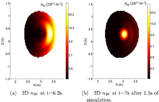
Figure 3. Poloidal cross sections of the W density inferred from SXR-UV measurements.
Download figure:
Standard image High-resolution imageThe measured profiles are fitted using the JET Profile Maker tool [18]. The only difference with the profiles used in [6] is that the profiles at the LCFS are here constrained by the measured data, the core profile fits being similar. Selection of electron density and temperature profiles obtained by cubic spline fits of the JET High resolution Thomson scattering (HRTS, time resolution of 50 ms) diagnostic are presented on figures 2(a) and (b). Note that the HRTS covers the axis. Through the whole time window, the pedestal height of the electron density fluctuates due to the presence of ELMs occuring at a frequency around 40 Hz, visible on the radiation on figure 1. At the beginning of our time window, the electron density profile is hollow at 5.5 s, which means that the density at ρ = 0.2 is lower than the density around mid-radius. The central density is already peaked. This phenomenon is most likely caused by NBI central particle source (see figure 18(a)) and low central diffusivity [19]. Then the density builds up over time from mid-radius inward, keeping a strong central peaking. One sawtooth crash occurs between 6.3 s and 6.5 s, causing the central density to drop. Between 6.8 s and 7.1 s the central density increases and then slightly drops again. As explained later on section 4, the density gradients, especially the central one, play a major role in W transport and central accumulation.
On figure 2(b), the electron temperature profiles remain quite unchanged from ρ = 0.3 outward. The central temperature tends to decrease over time, from ρ = 0.3 inward. The impact of the three sawtooth crashes (5.9 s, 6.5 s and 7.1 s) is visible: the central temperature increases between 6 s and 6.3 s, and again between 6.6 s and 6.8 s. Overall, the central electron temperature drops by 35% in 1.6 s.
On figure 2(c), the ion temperature profiles also undergoes the sawtooth crashes since the central temperature increases between 6 s and 6.3 s, but the inversion radius is less visible. Finally, the rotation profiles on figure 2(c) behave quite similarly to the ion temperature profiles with the increase/decrease due to the sawteeth. Note that the toroidal rotation is quite large, between 2.105 and 3.105 m · s−1, which leads to W Mach numbers up to 3.
The experimental W density has been calculated coupling data from the soft x-ray (SXR) diagnostic and vacuum-ultra-violet (VUV) spectroscopy using the method explained in [20] extended to account for poloidal asymmetries [21]. The obtained profiles over the time window studied here are similar to the ones analysed at two different times in [6]. They are shown on figure 3, at t = 6.2 s before the central SXR line on figure 1 peaks, and at t = 7 s during a SXR central line peak.
On figure 3(a) at t = 6.2 s, the W did not reach the center yet and gathers at the low field side (LFS), showing strong poloidal asymmetries as expected for rotating plasmas (see toroidal velocity profiles on figure 2(d)). At this time the W concentration on the LFS is around  so the W is still a trace species, i.e.
  . At 7 s shown on figure 3(b) a significant amount of W accumulated in the center of the plasma. The central W concentration reaches up
  therefore W is no longer a trace species.
The goal of this work is to model self-consistently the main features of the 82722 pulse: central electron density peaking, central electron temperature dropping, and W central accumulation by predicting with JETTO the time evolution of the plasma profiles (density, temperature, rotation) as well as the W profile.
3. JETTO configuration: codes, assumptions and numerical settings
The use of an integrated modeling tool is mandatory in order to evolve predictively many quantities at the same time: particles, heat, momentum as well as current and magnetic equilibrium. This section presents the JETTO configuration used for our specific case. Each code settings are briefly presented below, the corresponding numerical adjustments are shown in appendix.
JETTO is an integrated modelling plateform [22], where the heat, particle and angular momentum transport equations are solved over a chosen time period. Models for the sources are coupled to JETTO, as well as turbulent and neoclassical transport codes. In the JET pulse studied, only NBI is present, its associated heat, particle and angular momentum sources are modelled by PENCIL [23]. The turbulent transport in modelled by QuaLiKiz [15, 16] and the neoclassical transport by NEO [12, 13]. Our JETTO simulation evolves fully predictively, over several confinement times, seven channels: densities of main ions, W and Be, ion and electron temperatures, toroidal rotation, and current.
The time window, 5.5 s–7.1 s, was chosen to be wide enough to cover several confinement times (with  0.3 s with Wth the total energy of the plasma and PL the power loss) and at 7 s the W already accumulated in the center (see figure 3(b)). The entire plasma radius is modeled within JETTO. The overall JETTO settings are detailed in the appendix.
Figure 3(a) illustrates W strong poloidal asymmetries, making the use of a code accounting for poloidal asymmetries such as NEO necessary. NEO [24, 25] solves the full drift kinetic equation. It provides a first-principle calculation of the transport coefficients directly from the kinetic solution of the distribution function. It uses the full linearized Fokker–Planck multi-species collision operator. Within JETTO, NEO runs for the impurity neoclassical transport over the whole radius range, from the axis to the LCFS. NEO uses a Miller equilibrium [26] computed using general geometry information from JETTO.
For the turbulent transport, from  to the pedestal top
  , the quasilinear gyrokinetic code QuaLiKiz is used. It is a first-principle quasilinear gyrokinetic code that accounts for trapped and passing ions and electrons, therefore Ion and Electron Temperature Gradients and Trapped Electron Modes. QuaLiKiz produces quasilinear gyrokinetic heat, particle and angular momentum fluxes which have been successfully compared to non-linear gyrokinetic predictions [15, 27, 28]. QuaLiKiz handles shifted circular
  equilibrium, while JETTO maintains shaped flux surface geometry for all source calculations, and for setting the metrics in the transport PDEs. This necessitates certain choices and transformations when passing information between the codes. QuaLiKiz input are taken on each flux surface, except in presence of poloidal asymmetries where the LFS value is read. Concerning the gradients in QuaLiKiz, they are calculated along
  , where Rmax (respectively Rmin) is the maximum (respectively minimum) major radius of each flux surface. The QuaLiKiz output fluxes (per m2) are (circular) flux-surface-averaged, and the full flux surface area is used to calculate the total transport rates within JETTO. The effective diffusivities and heat conductivities calculated from these fluxes within QuaLiKiz are transformed into JETTO coordinates, using general geometry information from JETTO [16]. The impact of poloidal asymmetries for turbulent transport of heavy impurities is included, see a comparaison with GKW here [16]. QuaLiKiz accounts for all unstable modes and sums the fluxes over the wave number spectrum. Both QuaLiKiz and NEO codes are first-principle based and have a computational time compatible with integrated modelling (about 10 CPU seconds for a flux at a single radial location). Indeed, in JETTO, these transport codes are called at least 1000 times for each second of modelled tokamak plasma. More detailed NEO and QuaLiKiz settings inside JETTO are given in the appendix.
The pedestal region (ρ = 0.97–1) is modeled using an ad hoc 'edge transport barrier' (ETB), i.e. prescribed transport coefficients. The pedestal width and the turbulent transport remain fixed during the whole simulation. The code FRANTIC [29] models the neutral particle source at the LCFS. The transport coefficients and neutral particle source are tuned to reproduce the experimental Te and ne in this region within experimental uncertainties at all times. In the pedestal, the Prandtl number is also tuned to match the experimental rotation. A continuous ELM model, with tuned particle diffusivity and thermal conductivity was also necessary to reproduce the experimental pedestal, as in [30]. More details on the ETB settings in JETTO are given in the appendix.
The initial W density profile is fixed to be proportional to the electron density such that  allows to match both the experimental value of
  , and the initial line integrated radiation level from bolometry diagnostic within 5% (3.27 MW for experimental value of 3.41 MW). Concerning the W boundary conditions, a constant W fluence through the separatrix is fixed to 1015 part s−1. Therefore, the incoming W is transported through the pedestal with the neoclassical transport coefficients. Our aim here is to investigate if the core W accumulation can be captured while keeping a fixed W fluence through the LCFS fixed.
Concerning the magnetic equilibrium, the separatrix is determined by EFIT [31]. The current diffusion is self-consistently predicted in JETTO starting from an initial q profile given by EFIT constrained by the measured kinetic pressure and the Faraday angles [32].
The impurity radiative losses, as well as the impurity density profiles are computed by SANCO [17]. SANCO runs for the whole radius range, treats all charge states of the impurities. The atomic data used for W is ADAS 50, based on [33]. ADAS96 is used for Be. The SANCO settings in JETTO are further detailed in the appendix.
ELM crashes and sawteeth are not modeled in our specific case, although several models are available in JETTO/JINTRAC [30].
The heating source, in this case NBI only, is modeled using the PENCIL code [23]. PENCIL results were compared with NUBEAM in TRANSP [34] showing an agreement of the source profiles within 10%. PENCIL solves a simplified version of the Fokker-Planck equation and includes ionization by charge exchange, ionization by plasma electrons and ionization by plasma ions. PENCIL computes the NBI heat, particle and angular momentum sources. More details on the PENCIL seetings in JETTO are given in the appendix.
In the following, the above JETTO-SANCO-QuaLiKiz-NEO-PENCIL-FRANTIC-ETB settings will be run to solve the electron heat, ion heat, particle (D, W and Be) and angular momentum transport equations. In these equations, at each time step, the sources and the transport coefficients are recalculated, therefore they are evolved self-consistently over multiple time steps, at least 1000 per second, covering 5 confinement times (i.e. 1.7 s) of the JET H mode hybrid pulse #82722.
4. JETTO predictions versus experiments
In this section, we compare the experimental measurements with the self-consistently predicted profiles for the JET-ILW shot #82722 between 5.5 s and 7.1 s using JETTO-SANCO-QuaLiKiz-NEO-PENCIL-FRANTIC-ETB settings detailed in the previous section and in the appendix.
4.1. Time traces of the plasma parameters
Figures 4–9 present time traces of several plasma parameters which are self-consistently and simultaneously evolved in the simulation: density, temperature, rotation, current profiles as well as impurity content and radiation. For each parameter, the JETTO-SANCO-QuaLiKiz-NEO-PENCIL-FRANTIC-ETB simulation is shown in magenta, and compared with experimental measurements when available. Timetraces are shown at three ρ positions: 0.1, 0.4, and 0.75.
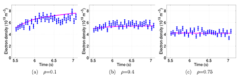
Figure 4. Electron density time traces: comparison between JETTO-SANCO-QuaLiKiz-NEO-PENCIL-FRANTIC-ETB prediction (full line, magenta) and HRTS measurements (blue crosses with the uncertainties on the measurement) at different normalized radius, ρ.
Download figure:
Standard image High-resolution image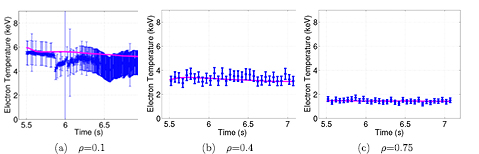
Figure 5. Electron temperature time traces: comparison between JETTO-SANCO-QuaLiKiz-NEO-PENCIL-FRANTIC-ETB prediction (magenta, full line) and ECE at  /HRTS measurements at
  (in blue).
Download figure:
Standard image High-resolution image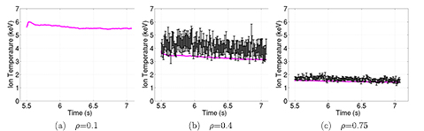
Figure 6. Ion temperature time traces: comparison between JETTO-SANCO-QuaLiKiz-NEO-PENCIL-FRANTIC-ETB prediction (full line magenta) and Charge Exchange measurements (black crosses, with their uncertainties) at different normalized radius, ρ.
Download figure:
Standard image High-resolution image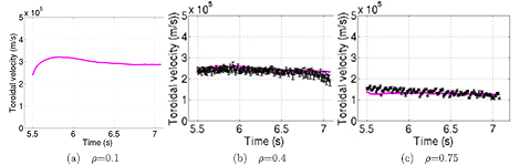
Figure 7. Toroidal rotation timetraces: comparison between JETTO-SANCO-QuaLiKiz-NEO-PENCIL-FRANTIC-ETB prediction (magenta) and Charge Exchange measurements at different (in black).
Download figure:
Standard image High-resolution image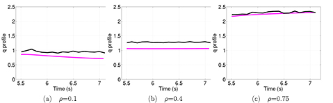
Figure 8. Safety factor timetraces: comparison between JETTO-SANCO-QuaLiKiz-NEO-PENCIL-FRANTIC-ETB prediction (magenta) and EFIT reconstruction constraint by the measured kinetic pressure and the Faraday angles [32] (in black) at different ρ.
Download figure:
Standard image High-resolution image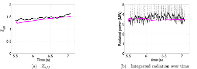
Figure 9. Zeff and radiation timetraces: comparison between JETTO-SANCO-QuaLiKiz-NEO-PENCIL-FRANTIC-ETB prediction (magenta) and measurements at different (in black) ρ.
Download figure:
Standard image High-resolution imageFigure 4 shows the time evolution of electron density. The density prediction must be accurate in order to simulate properly the W transport, due to the main ion density gradient dependence of the W neoclassical transport (see equation (2) of [35]). On figure 4(a), close to the center, the predicted density increases smoothly. The HRTS measurements, while also globally increasing, are impacted by the sawteeth. The simulation does not take sawteeth into account, therefore the local gradients are not well captured at all times. For the two other radial positions, the predicted density does not vary much, and mostly stays within experimental uncertainties.
Figure 5 shows the electron temperature. Similarly to the electron density case, the simulation successfully captures the decreasing trend of central ECE measurements on figure 5(a), but expectedly misses the sawtooth crashes. Around mid-radius (figure 5(b)) and close to the pedestal (figure 5(c)), the experimental temperature remains quite steady and the predictions lie within experimental uncertainties over time.
Ion temperature and toroidal rotation are not compared with experimental data in the center (figures 6(a) and 7(a)) due to lack of charge exchange data there. At  on figure 6(b), the predictions tend to underestimate the charge exchange measurements by at most 15% (calculated from the lower bound of the error bar). A potential source for this Ti underestimation is the lack of electromagnetic stabilization of ITG turbulence [36] in the electrostatic QuaLiKiz model. Indeed, the pulse studied here is a high-performance hybrid H-mode, where electromagnetic stabilization is typically more prominent due to high-β and reinforced by a high fast ion fraction, as shown by nonlinear gyrokinetic simulations for a JET hybrid pulse in [37].
Toroidal rotation predictions mostly lie within experimental uncertainties, except at early times at  . Overall, the experimental toroidal velocity remains quite constant over time. Note that the plasma rotates up to 300 km s−1, which leads to a W Mach number up to 3 leading to strong poloidal asymmetries.
The predictions of safety factor evolution are shown on figure 8. The self-consistent current diffusion equation solved in JETTO leads to these predictions of q. This predicted q differs slightly from the EFIT reconstruction constrained by kinetic pressure and Faraday angles [32].
Figure 9(a) shows the average Zeff time evolution and figure 9(b) shows the total radiated power over time. The Zeff globally increases with time, which can be explained by the fact that W contribution to Zeff increases also with time. The line integrated radiated power does not increase over time, nor in the experiment neither in the simulation. The simulation does not account for ELMs, therefore it does not capture the regular bursts reported on the bolometer signal. The fact that the W core accumulation is not visible on the line integrated bolometer signal is due to the fact that the W cooling factor is maximum around T = 1.5 keV [33], hence off-axis for the pulse studied here.
Figure 10 shows the time evolution of the W content. The simulation values are renormalized to  , i.e the time average of the ratio of the simulation value over the measurement value at
  and
and  . Importantly, note that flux surface averaged and 2D W profiles are compared without renormalization on figures 15–17. The initial W content was estimated from the total radiation shown on figure 9(b). Due to uncertainties, some experimental values are unavailable. In the very core,
  , the simulated W density slowly and regularly increases, with a factor 3 increase between 6 s and 7 s. The W density inferred from SXR-UV measurements [20] accumulates a little at 6.3 s before being flushed out by the second sawtooth. Between the second and the third sawtooth, from 6.7 s, the core W rises by a factor 10. The JETTO-SANCO-QuaLiKiz-NEO-PENCIL-FRANTIC-ETB simulation, which does not account for sawteeth, captures the core W accumulation trend. The predicted W content at
  and
and  are compared to the measured ones in figures 10(b) and (c). Note that in a JETTO-NEO simulation, where all the channels where run interpretatively but W transport which was predicted by NEO, a much better agreement of the W time evolution was obtained. This demonstrates that the mismatch in the temporal evolution of W is due to the difference in the predicted versus interpreted density, rotation and temperature profiles, not due to the W transport modelling.
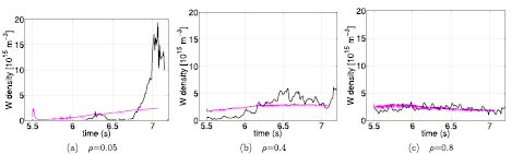
Figure 10. W density timetraces: comparison between JETTO-SANCO-QuaLiKiz-NEO-PENCIL-FRANTIC-ETB prediction (magenta) and estimation from SXR-UV measurements (black) at different ρ at  . Here the simulation values are renormalized to the time averaged ratio:
  .
.
Download figure:
Standard image High-resolution imageTo deepen the analysis of the quality of the JETTO-SANCO-QuaLiKiz-NEO-PENCIL-FRANTIC-ETB predictions, the next subsection focuses on several profiles at different time slices, and 2D poloidal cuts of the W distribution.
4.2. Plasma profiles
4.2.1. Electron density.
In order to further validate QuaLiKiz predictions, figure 11 shows electron density profiles at three different times: 6.2 s after 0.7 s of simulation (figure 11(a)), 6.8 s after 1.3 s of simulation (figure 11(b)) and 7 s, after 1.5 s of simulation (figure 11(c)). Both HRTS and LIDAR are shown on figure 11 but we shall compare the simulation with HRTS only because of its higher time and space resolutions.

Figure 11. Comparison of experimental (LIDAR in black HRTS in blue) and predicted (magenta solid line) electron density profiles.
Download figure:
Standard image High-resolution imageOn figure 11(a) at 6.2 s, QuaLiKiz predictions in magenta lie within experimental uncertainties of the HRTS in blue for the whole radius, except close to the axis where QuaLiKiz misses the local variations. The predicted pedestal is modeled by the ETB which has been tuned to match the experimental data. On figure 11(b) at 6.8 s, QuaLiKiz prediction lies within experimental uncertainties from R = 3.3 m outward. But from R = 3.3 m inward, the experimental density dropped because of a sawtooth, therefore QuaLiKiz overestimates the central electron density. The experimental pedestal is stable and well captured by the edge transport barrier modeling. On figure 11(c) at 7 s after 1.5 s of simulation, HRTS shows strong local gradients, especially close to the axis at R = 3.1 m. The experimental pedestal is slightly shifted outward, therefore the Edge Transport Barrier no longer lies within experimental uncertainties. QuaLiKiz captures the global increase of the electron density and lies within experimental uncertainties. However it does not fully reproduces the stiff central gradient shown by the measurements. This impacts the W transport as seen in the next section, and could be improved in the future by including a sawtooth model.
4.2.2. Electron and ion temperatures.
The electron and ion temperature predictions are then compared with experimental data. The electron temperature profiles are first shown on figure 12: at 6.2 s after 0.7 s of simulation (figure 12(a)), at 6.8 s after 1.3 s of simulation (figure 12(b)) and at 7 s after 1.5 s of simulation (figure 12(c)). QuaLiKiz predictions are in magenta solid line, and the HRTS measurements in blue.

Figure 12. Comparison of experimental (HRTS in blue) and predicted (magenta solid line) electron temperature profiles.
Download figure:
Standard image High-resolution imageOn figure 12(a) at 6.2 s, QuaLiKiz predictions of Te in magenta lie within experimental uncertainties of the HRTS measurements in blue accross the whole radius, except at R = 3.3 m where QuaLiKiz misses a bump in Te and slightly underestimates the measurements. On figure 12(b) at 6.8 s, the HRTS shows a global decrease of the electron temperature, while keeping the central peaking and the bump at R = 3.3 m. The experimental pedestal remains unchanged and is well reproduced by the Edge Transport Barrier. QuaLiKiz predicts the global decrease of the electron temperature, but still misses the bump at R = 3.3 m. QuaLiKiz predicts the central peaking and slightly overestimates it. On figure 12(c) at 7 s after 1.5 s of simulation, the bump at R = 3.3 m disappears while a drop appears at R = 3.5 m. QuaLiKiz predictions barely change compared with 12(b). Therefore it misses the drop at R = 3.5 m while staying within experimental uncertainties. QuaLiKiz still overestimates the very central temperature.
Now the ion temperature profiles are shown on figure 13: at 6.2 s after 0.7 s of simulation (figure 13(a)), at 6.8 s after 1.3 s of simulation (figure 13(b)) and at 7 s after 1.5 s of simulation (figure 13(c)). QuaLiKiz predictions are in magenta solid line, and the charge exchange measurements are in black for most of the radial points, and blue for the pedestal.
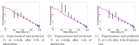
Figure 13. Comparison of experimental (charge exchange in dark) and predicted (magenta solid line) ion temperature profiles.
Download figure:
Standard image High-resolution imageOn figure 13(a) at 6.2 s, QuaLiKiz predictions in magenta lie within experimental uncertainties of the Charge Exchange measurements for the whole radius. On figure 13(b) at 6.8 s, the Charge Exchange measurements show a global increase of the ion temperature, up to 50% at R = 3.2 m. QuaLiKiz predictions remain almost unchanged and therefore underestimates the measurements by a maximum of 15% (calculated from the lower bound of the error bar). The possible reasons for this underestimation were developed in the previous section. On figure 13(c) at 7 s after 1.5 s of simulation, measured ion temperature slightly decreases at R = 3.25–3.4 m. QuaLiKiz predictions barely change compared with figure 13(b). Therefore it still underestimates the measurements at R = 3.25–3.4 m.
4.2.3. Rotation.
The last plasma parameter to study is the toroidal rotation, shown on figure 14: at 6.2 s after 0.7 s of simulation (figure 14(a)), at 6.8 s after 1.3 s of simulation (figure 14(b)) and at 7 s after 1.5 s of simulation (figure 14(c)). QuaLiKiz predictions are in magenta solid line, and the Charge Exchange measurements are in black for most of the radial points, and blue for the pedestal.

Figure 14. Comparison of experimental (charge exchange in dark) and predicted (magenta solid line) toroidal rotation profiles.
Download figure:
Standard image High-resolution imageOn figure 14(a) at 6.2 s, QuaLiKiz predictions in magenta lie within experimental uncertainties of the Charge Exchange measurements for the whole radius. The central part also lacks experimental measurements. On figure 14(b) at 6.8 s, the charge exchange measurements show a slight global decrease of the toroidal rotation, especially at R = 3.5–3.65 m. QuaLiKiz predicts the global decreasing but overestimates the strongest decrease of the measurements at R = 3.5–3.65 m. Finally, on figure 14(c) at 7 s after 1.5 s of simulation, measured velocity profile moves slightly. QuaLiKiz predictions barely changed compared with 14(b). Therefore it slightly overestimates the measurements at R = 3.3–3.7 m and the edge transport barrier model, which does not evolve, misses the pedestal.
4.3. W profiles and poloidal cuts
To analyze more precisely the time evolution of the W profile, figure 15 shows the Flux Surface Averaged W profiles at t = 6.2 s after 0.7 s of simulation and t = 7.1 s after 1.6 s of simulation. The experimental data is not available from  outwards where the SXR signal is too weak to constrain the W profile reconstruction. Note that here, unlike for figure 10, the profiles are not renormalized one to the other. And also note that, unlike previous works [6, 7], where each 2D nW prediction was independently normalised to SXR, here the W content is, for the first time predicted in absolute value.
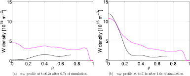
Figure 15. Comparison of profiles of estimated W density from SXR-UV measurements (black) and predicted W density (magenta) flux surface averaged.
Download figure:
Standard image High-resolution imageAt 6.2 s on figure 15(a), the simulation overestimates the W content inferred from measurements by a factor 2 at mid-radius and up to a factor 10 in the very center where, according to the experimental data, the W did not migrate yet. This discrepancy probably comes from the initial condition which constrains the W profile to be homothetic to the electron density profile. At 7.1 s, after 1.6 s, on figure 15(b), the simulated central W content is very similar to the data inferred from SXR measurements, hence capturing the W core accumulation. The simulation still slightly overestimates the measurements from  outward.
Figures 16 and 17 show 2D maps of the W density at two different times: t = 6.2 s after 0.7 s of simulation and t = 7 s after 1.5 s of simulation. W densities estimated from SXR-UV measurements are on the right, predictions are on the left.

Figure 16. Comparison of estimated W density from SXR-UV measurements (right) and predicted W density (left) at t = 6.2 s after 0.7 s of simulation.
Download figure:
Standard image High-resolution image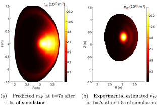
Figure 17. Comparison of estimated W density from SXR-UV measurements (right) and predicted W density (left) at t = 7 s after 1.5 s of simulation.
Download figure:
Standard image High-resolution imageOn figure 16, one can see that the W density, both measured and simulated is in the  range. The initial amount of W was homothetic to the electron density profile, which is very different from experiment (see figure 15(a)). Therefore, in the simulated profiles, there is W in the very core from the start, unlike the experiments. Concerning poloidal asymmetries, at 6.2 s, both the measured and the simulated profiles show strong poloidal asymmetries, although they are weaker in the predicted profiles.
At the end of the simulation, after 1.5 s at t = 7 s, the estimation from measurements on figure 17(b) shows that most of the W moved towards the center and accumulated. On the simulation, most of the W kept moving towards the center, but not fast enough and a significant W amount is still present at mid radius (see figures 10(b) and (c)). However the time evolution of the W behavior definitely shows a trend of core accumulation.
Three phenomena can explain why the simulation does not fully succeed in transporting all the W to the plasma center. The first explanation is that the simulation does not model sawteeth and therefore some transport mechanisms can be missed. The second explanation is that the initial W profile, with some W already in the center and at mid-radius unlike the experiment, remains present even after a few confinement times. The third explanation could be that QuaLiKiz, as seen on figure 11 globally captures the global central density peaking but does not fully reproduce all the local gradients, especially at mid-radius and in the center. This could lead to underestimated neoclassical transport and therefore a weaker central accumulation.
Overall, the accuracy of the QuaLiKiz predictions of the main plasma profiles, especially electron density and rotation, allows NEO and QuaLiKiz to correctly estimate the W neoclassical transport and therefore reproduce the W central accumulation trend even though more work is required to capture all the experimental features of the background profiles, in particular the sawteeth impact on them.
5. Actuators to avoid W central accumulation
The simulation predicts self-consistently and simultaneously the plasma profiles evolution, as well as the W tendency for central accumulation. In this section, the actuators leading to the accumulation are studied. According to the equation of the neoclassical W flux from [35], three main physical parameters impact the W neoclassical flux: the main ion temperature profile, the main ion density gradient and W poloidal asymmetries. Both the ion density and the level of poloidal asymmetries can be modified through the NBI injection: the first one via the position of the NBI particle fuelling, the second is linked with the NBI angular momentum input.
5.1. Central particle fuelling
According to equation (2) of [35], in the case of an inward W particle flux, a larger main ion density gradient leads to a larger inward W neoclassical flux. In the case of 82 722, the particle fuelling is stronger in the central part (see figure 18(a)), causing the particle density to peak (figure 4(a)).

Figure 18. Study of the impact of central NBI particle source on W core accumulation. Reference simulation (magenta), simulation with NBI particle source at zero (blue) and partial-off axis particle souce (red).
Download figure:
Standard image High-resolution imageIn order to confirm the link between central particle fuelling and central W accumulation, two new simulations are set: one with the particle injection artificially set to zero in PENCIL settings at all times; and the other with partial off-axis particle source at all times. In all cases, only the PENCIL NBI particle source is modified, the NBI heating and angular momentum input are kept identical to the original simulation. Figure 18(a) illustrates the NBI particle source profiles at 6.5 s for the three cases.
Figure 18(b) shows the W density Flux Surface Averaged over time at ρ = 0.05. The shaded section on figure 18(b) from t = 5.5 s to t = 5.7 s corresponds to the first simulated confinement time, needed for the simulation to move away from initial conditions. The removal of the central density source completely mitigates the W accumulation phenomenon. With a 45 % reduction of the central particle source, the central W density is reduced by 42%. Figure 18(c) shows the W density Flux Surface Averaged profile at t = 6.5 s. Without the central particle source, there is almost no W in the central part, most of the W is located in the outer half. The W density profiles of the reference simulation and the simulation with partial off-axis particle fuelling are quite similar from ρ = 0.4–1, but in the center, the partial off-axis particle fuelling reduces the W central accumulation by 45%.
When switching off, or reducing the particle source, the background plasma profiles are impacted as well. This is illustrated on figure 19 for the density, temperatures and rotation profiles at t = 6.5 s. As expected, the removal on the central particle fuelling annihilates the central electron density peaking. The reduction of central fuelling by  in red leads to a reduction of the central density peaking by only
  . Since without central particle fuelling, W does not accumulate, larger temperatures are obtained in absence of core particle fuelling.
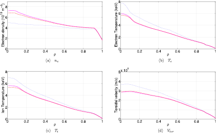
Figure 19. Density, temperatures and toroidal rotation profiles at t = 6.5 s. Reference simulation (magenta), no NBI particle source (blue), partially off-axis NBI particle source (red).
Download figure:
Standard image High-resolution imageOverall, this study demonstrates the deleterious correlation between NBI central particle fuelling and the W central accumulation. This is encouraging for devices such as WEST or ITER, with off-axis particle fuelling.
5.2. NBI angular momentum impact
The other parameter impacting significantly the W neoclassical transport is the rotation. The impact of poloidal asymmetries in the W neoclassical transport is accounted for in the geometrical terms PA and PB in equation (2) of [35], and their range of applicability is studied in [38]. In this specific rotating JET-ILW pulse, these geometrical factors enhance the neoclassical convection up to a factor 40. In order to study the impact of rotation on the W central accumulation, a simulation is set with the NBI angular momentum set to zero while keeping identical the heat and particle sources. The resulting torque, and core W density evolution are illustrated on figure 20.
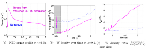
Figure 20. Study of the impact of toroidal velocity on W core accumulation. Reference simulation (magenta) versus simulation with toroidal rotation at zero (blue).
Download figure:
Standard image High-resolution imageOn figure 20(b), during the first confinement time in the shaded area, for the reference simulation in magenta, the central W content drops before increasing again. Indeed W density profile equilibration time scale is much shorter than the energy confinement time scale. The removal of the NBI angular momentum makes the W transport much more sensitive to the initial condition. However, for the simulation with no torque, the W content remains stable and then increases. This makes the two simulations not directly comparable. In order to remove the effect of the first confinement time on W density, figure 20(c) shows the timetrace of W density normalized to its value at the end of the first confinement time, at t = 5.7 s. Without NBI angular momentum, W central content doubles over time, while in presence of toroidal rotation, the W density increases by a factor 10. This clearly illustrates that the toroidal rotation plays a role in the W central accumulation process.
The removal of the NBI angumar momentum causes the two simulations to have very different early phases and therefore completely different time evolutions. We shall focus on the first confinement time in order to understand the mechanisms leading to such a big difference.
As mentioned earlier, the initial W density profile is homothetic to the electron density profile, therefore some W is already present in the center at the start. In absence of NBI torque, the W is equally poloidally distributed along each flux surface which reduces significantly its neoclassical inward convection. Figure 21 shows the W transport coefficients at the end of the first confinement time, at t = 5.7 s, time averaged over 0.1 s to smooth the QuaLiKiz predictions.
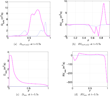
Figure 21. W transport coefficients at t = 5.7 s, time averaged over 0.1 s. Reference simulation (magenta), no toroidal rotation (blue).
Download figure:
Standard image High-resolution imageAs expected, the removal of the torque reduces by a factor PA, the neoclassical diffusion and convection (on figures 21(c) and (d)). The neoclassical convection is strongly reduced both in the very core and in the pedestal region.
The absence of torque also reduces the turbulent effective convection and diffusion for  by up to a factor 10. Note that the outputs to JETTO are either a
  or a
or a  , depending on the direction of the transport and the size of the gradient. Therefore there are radial regions of zero
  that have non-zero
  , and since it is averaged over 0.1 s, in some cases both
  and
and  can be at play. The impact of poloidal asymmetries on W turbulent transport is accounted for in QuaLiKiz based on [39], as described in [16]. The impact of centrifugal effects on the various components of the turbulent convection (thermodiffusion, rotodiffusion, pure convection) results of a complex compensation of the different components (see [39]) leading, in this case, to a reduced turbulent W transport in absence of torque.
Overall, in absence of NBI torque, both turbulent and neoclassical W transport are reduced. As a consequence, W is no longer flushed out from the central zone of the plasma over the first confinement time. During the rest of the simulation, it is weakly transported to the center by residual neoclassical convection, but the W amount transported is negligible in absence of NBI angular momentum compared with the case with NBI torque (see figure 20(c)).
When removing the NBI torque, the turbulent main ions heat and particle fluxes are also affected (see [40] for details on the  implementation in QuaLiKiz). Figure 22 shows the heat fluxes profiles from JETTO simulations (reference and without rotation) at t = 5.7 s, after the first confinement time. When setting to zero the torque, the
  shear is largely reduced [41]. Due to a weaker
  shear, the heat coefficients are larger in absence of torque. As a consequence, the electron and ion temperatures are lower in, as seen on figures 23(b) and (c). Note that the electron density profile on figure 23(a) is weakly impacted, except for the central density peaking which is slightly higher in absence of torque. The central radiation on figure 23(d) is larger in absence of torque since the W is not flushed out.
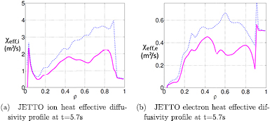
Figure 22. Ion and electron heat effective diffusivities profiles from JETTO simulations at t = 5.7 s: reference (magenta) and without rotation (blue).
Download figure:
Standard image High-resolution image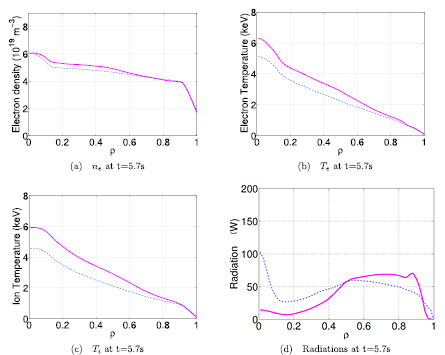
Figure 23. Density, temperatures and radiation profiles at t = 5.7 s. Reference simulation (magenta), no toroidal rotation (blue).
Download figure:
Standard image High-resolution imageIn summary, the removal of the NBI angular momentum strongly reduces the W neoclassical convection, as expected, and also its turbulent transport (see figure 21). But removing the torque leads to more unstable background plasma heat and particle transport (see figures 22(a) and (b)). Initially, the removal of the rotation is deleterious for both the energy confinement (increased turbulence for main ion and electrons) and the central W content since W is no longer flushed out. But once the impact of the initial condition removed, it appears that NBI torque has a negative impact on the W central accumulation (see figure 20(c)). Therefore lower torque experiments, such as WEST or ITER, should be less prone to core W accumulation.
6. Non-linearities: W stabilization impact
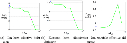
A simulation evolving self-consistently particle, heat, momentum for electrons, ions and impurities (W and Be) involves numerous non-linearities. One of these features is illustrated by the fact that removing the W from our reference simulation leads to a slightly lower total energy content, see figure 24(d). In the simulation with Be only, the Zeff is still 1.34 as in the reference. When removing the W while keeping Zeff constant, the lower energy content is explained by a higher ion heat effective diffusivity, see figure 24(a), while maintaining similar electron heat and ion particle effective diffusivities, see figures 24(b) and (c).
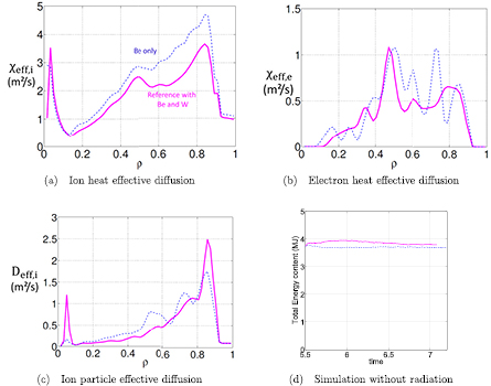
Figure 24. Ion and electron heat effective diffusion and ion particle effective diffusion profiles at t = 6.5 s, and timetrace of the total energy content. Reference simulation with W and Be (magenta) and simulation with Be only (blue).
Download figure:
Standard image High-resolution imageRemoving the W from our reference simulation impacts the radiation level, the plasma effective charge, hence its collisionality and the ITG drive.
6.1. Possible cause: radiation
When removing the W from our reference simulation the radiation level is almost reduced to zero. Therefore to isolate the impact of radiation from the impact of the W itself, a simulation as our refernce case but with the radiation forced to zero is run.
It is interesting to note that the energy content of the Be only case and W-Be but no radiation case are very similar (within 1%), see figure 25(d). When comparing the effective ion heat diffusivities, removing the radiation from the reference case is destabilizing for  , see figure 25(a). A similar impact is seen also on the electron heat effective diffusivity, figure 25(b), as well as on the ion particle effective diffusivity, figure 25(c).

Figure 25. Ion and electron heat effective diffusion and ion particle effective diffusion at t = 6.5 s, and timetrace of the total energy content. Reference simulation with W and Be (magenta), simulation with Be only (blue) and simulation with Be and W without radiation (red).
Download figure:
Standard image High-resolution imageIn order to have a better understanding of the stabilization effect, the timetraces of ion and electron temperatures, the ratio  and the ion heat diffusivity are shown on figure 26 for the position ρ = 0.7.
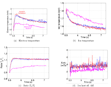
Figure 26. Ion and electron temperatures, ratio  and ion heat effective diffusion timetraces at ρ = 0.7. Reference simulation with W and Be (magenta), simulation with Be only (blue) and simulation with Be and W without radiation (red).
Download figure:
Standard image High-resolution imageThe curves split in two groups: the reference simulation with W and radiation on one side (magenta), and the simulations without radiation either with or without W on the other side. Without radiation, as expected, the electron temperature on figure 26(a) is higher. The ion temperature on figure 26(b) is also impacted and is lowered. The modification in the temperature impacts the ratio  shown on figure 26(c), which is higher for the simulations without W radiation.
The enhanced electron temperature, combined with lower ion temperature leads to enhanced  , which is known to increase ITG dominated turbulence [27]. Therefore, the destabilization effect could be explained by this mechanism: the removal of W causes the radiation level to be significantly reduced, leading to an enhanced
  , causing the turbulence to be increased. In order to validate this explanation, a QuaLiKiz stand-alone simulation is run, scanning the electron temperature. All the other inputs are taken from the JETTO reference simulation parameters at t = 6.5 s and ρ = 0.7. The profile values entered as input in QuaLiKiz are taken on each JETTO flux surface (except the W density taken at the outboard mid-plane) and the gradients are calculated along
  , where Rmax (respectively Rmin) is the maximum (respectively minimum) major radius of each flux surface. The ion and electron heat effective diffusivities and the ion particle effective diffusion are shown on figure 27. The red diamond corresponds to the
  ratio at t = 5.7 s at ρ = 0.7 for the simulation without radiation, in red on figure 26. The magenta circle corresponds to the
  ratio at t = 5.7 s and at ρ = 0.7 for the reference simulation. Note that JETTO is an iterative flux driven process while in QuaLiKiz stand-alone the gradients are kept fixed.
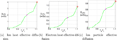
Figure 27. QuaLiKiz stand-alone: ion and electron heat effective diffusion and ion particle effective diffusion at t = 6.5 s.
Download figure:
Standard image High-resolution imageOn figures 27(a) and (b), ion and electron heat effective diffusivities both increase with the ratio  , as expected. It is coherent with the JETTO simulation, figure 26. Note that the slope of the increase of heat coefficients is quite stiff. As a consequence, a small modification of the
  ratio impacts significantly the turbulence. In this case, the removal of the radiation (i.e. the variation of heat diffusion between the red diamond and the magenta circle) caused an increase of 2.0
  for the ion heat diffusion, 0.54
  for the electron heat coefficient and 0.61
  for the ion particle diffusion coefficient.
The removal of the radiation impacts the temperature and has a destabilizing effect. This indicates that a significant portion of the stabilization phenomenon occurs through the radiation. The next section focuses on the other mechanism susceptible to have a stabilizing effect: the combined effect of Zeff stabilizing impact on ITG and increased collisionality.
6.2. Other possible causes: Zeff stabilizing impact on ITG and increased collisionality
The other mechanisms that could participate to the stabilization effect of W, are the combination of Zeff stabilizing impact on ITG [42] and increased collisionality. Indeed, even if W is a trace impurity, it undergoes poloidal asymmetries and therefore can locally no longer be a trace species. Figure 28 shows the 2D poloidal cut of the W contribution to the Zeff at t = 6.5 s as an illustration. The W contribution to Zeff remains similar at all times of the simulation.
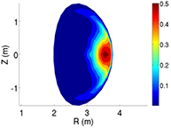
Figure 28. W contribution to the effective charge  at t = 6.5 s.
Download figure:
Standard image High-resolution imageOn the LFS, the poloidal asymmetries cause the W to contribute to Zeff up to 0.5. In those zones, the W is no longer a trace species and can contribute to the ITG stability as well as modify the collisionality. Since the interchange ITG-TEM modes are ballooned on the low field side, where the W contribution to Zeff is maximal it can indeed locally stabilize the turbulence [27, 42–44]. Moreover, W locally contributes to collisions, causing electrons to be untrapped and therefore lowering the TEM contribution. Both those effects caused by W can stabilize turbulence.
Using QuaLiKiz in stand-alone, the W concentration (calculated along  as the other input data) is increased and its impact on the effective diffusivities is illustrated by figure 29. The blue star corresponds to the zero W concentration for the simulation with Be only, in blue on figures 25. The magenta circle corresponds to the W concentration at t = 6.5 s at ρ = 0.7 for the reference simulation.
Figure 29. QuaLiKiz stand-alone: ion and electron heat effective diffusion and ion particle effective diffusion at t = 6.5 s.
Download figure:
Standard image High-resolution image
On figures 29(a) and (b), ion and electron heat effective diffusivities remain unchanged until they reach a  of ≃0.3. On figure 29(c), the main ion particle effective diffusivity follows a different trend, as it includes both the convective and diffusive contributions. The values of transport coefficients between the case without W and the W concentration from reference JETTO simulation (ie the difference between the blue star and the magenta circle) are of 3.1
  for the ion heat diffusion, 0.97
  for the electron heat coefficient and 0.62
  for the ion particle diffusion coefficient. Therefore the contribution of the effective charge to the heat transport stabilization effect is 30% bigger compared to the contribution through the radiation impact illustrated on figure 27.
Overall, the W has a stabilizing effect on the turbulence. The effect occurs through radiation and the modification of temperature profiles, but also through the effective charge impact on ITG and collisionality.
7. Conclusions and outlook
Overall, for the first time, an integrated, flux driven, core transport simulation evolves 7 channels (current, ion and electron temperatures, main ion Be and W densities and rotation profiles) over multiple confinement times. Within the integrated modeling environment JETTO, first-principles codes such as QuaLiKiz and NEO model respectively turbulent and neoclassical transport, up to the pedestal top. An empirical model is tuned to reproduce experimental measurements in the pedestal. The NBI particle, heat and sources are self-consistently modeled using PENCIL, while SANCO evolves the radiation levels.
The simulation successfully reproduces the time evolution over 1.5 s (hence 5 confinement times) of the temperature, density and rotation profiles. Moreover, the W tendency for central accumulation is captured by the simulation of turbulent and neoclassical transports, while keeping a constant W fluence at the separatrix over time. Indeed, for this modelled pulse, the W fluence is very small relative to total W content which is almost constant, i.e. our modelling shows that in this pulse the ELM flushing and inter ELM inward pedestal convection are in balance. In future work, in order to improve the W profile prediction, the initial 2D W profile should be closer to the one inferred from SXR and UV measurements, and more importantly, a sawtooth model should be applied in JETTO to mimic the background temperature and density crashes as done in [30]. The impact of such crashes on the subsequent W transport would be modelled self-consistently by NEO and QuaLiKiz. Finally, to improve further the predictability, a physically constrained pedestal, for example by EPED [45], should be activated in JETTO as done in [30].
Actuators of the W core accumulation are studied. It appears that removing the central NBI particle source cancels the central W accumulation, and cutting by half the central particle fuelling reduces also by half the W central accumulation. The suppression of the torque reduces the neoclassical W transport as expected, but also reduces the W turbulent transport. In this case, switching off the toroidal rotation has a destabilizing impact on the main ion and electron turbulence, and a stabilizing impact on the W transport. Therefore the W remains in the plasma center, however the accumulation is weaker. Note that, in Alcator C-Mod, W laser-blow off experiments, in presence of RF only, showed no sign of core accumulation [9]. This is also encouraging for devices such as WEST or ITER, which will operate without external torque, and without central particle fuelling.
Finally, it is observed that the presence of W has a stabilizing impact and leads to slightly higher energy content. Indeed, through radiation, the presence of W leads to lower  which stabilizes ITG turbulence. Moreover, on the low field side, because of W poloidal asymmetries in a rotating plasma, the W contribution to Zeff at the outboard mid-plane can go up to 0.5. This Zeff increment is also stabilizing the ITG turbulence. Nonetheless, these interesting impacts of W on the confinement are not sufficient to compensate for the deleterious impact of W core accumulation.
This integrated modelling work, accounting for all transported channels, including highly radiative impurities, has to be continued: to model existing experiments on JET, AUG, WEST and EAST; to optimize the scenarios in these exiting tokamaks; to predict ITER scenarios and also to predict the highly radiative DEMO scenario, where Xe injection if foreseen [46]. For a more intensive and systematic use of such complete integrated modelling, the transport codes have to become even faster. To this aim a Neural Network version of QuaLiKiz is being developed [47, 48]. It has recently been implemented in RAPTOR for control-oriented temperature and density profile prediction [49]. At a later stage, it is planned to extend the neural network modelling towards heavy impurity content control.
Acknowledgments
This work has been carried out within the framework of the EUROfusion Consortium and has received funding from the Euratom research and training programme 2014–2018 under grant agreement No 633053. The views and opinions expressed herein do not necessarily reflect those of the European Commission.
Appendix
A.1. JETTO numerical settings
JETTO settings:
| Shot number | 82722 |
| Number of grid points | 61 |
| Start time (s) | 5.5 |
| End time (s) | 7.1 |
| Minimum timestep (s) | 10−8 |
| Maximum timestep (s) | 10−3 |
| Ion (1) mass | 2 |
| Current boundary condition (amps) |  |
| Electron temperature boundary condition (eV) | 102 |
| Ion temperature boundary condition (eV) | 102 |
Ion density boundary condition ( ) ) |
 |
| Edge velocity boundary condition (cm s−1) | 106 |
| Grid resolution for QuaLiKiz | 25 |
SANCO settings:
| Tungsten | Berylium | |
|---|---|---|
| Impurity mass | 184 | 9.0129 |
| Impurity charge | 74 | 4 |
| Escape velocity (cm s−1) | 0 | 0 |
| Neutral flux (s−1) | 1015 | 1014 |
| Recycling factor | 0 | 0 |
| Abundance | 1 | 300 |
| Ratio SANCO/JETTO timestep | 100 | 100 |
NEO settings:
| Radial grid | 16 |
| Pitch angle polynomials | 13 |
| NEO transport update timestep (s) | 2.10−4 |
QuaLiKiz settings:
 |
0.03 |
 |
0.97 |
Impact of  , ,  and and  |
Only for  |
 range range |
ITG-TEM scales, ETG not taken into account here |
| Added diffusion coefficient | a Bohm diffusion of 0.1% of the particle diffusion coefficient, |
| To ensure numerical stability | 1% a Bohm–GyroBohm heat diffusion coefficient [50] |
ETB settings:
| Pedestal width (cm) | 4 |
| Lower thermal limit (cm2 s−1) | 5.103 |
| Lower particle ion limit (cm2 s−1) | 1.103 |
| Top of barrier FRANTIC gas puff target (cm−3) | 4.5.1013 |
| Top of barrier FRANTIC ion nominal puff rate (s−1) | 6.1021 |
| FRANTIC recycling coefficient | 0.1 |
| ELM model max. transport multiplier (m2 s−1) | 1.108 |
| Prandtl number for ETB | 0.75 |
PENCIL settings:
| Octant 4 | Octant 8 | |
|---|---|---|
| Ion mass | 2 | 2 |
| Ion energy (keV) | 90 | 97 |
| Beam fraction with E, E/2, E/3 | 0.51, 0.28, 0.21 | 0.52, 0.30, 0.18 |
| Pini's | 1, 4, 6 | 1, 4, 6 |
| Normalize power to (MW) | 6 | 10 |