


Abstract
A large eddy simulation (LES) approach is introduced to enable the study of the nonlinear growth of ballooning modes in a heliotron-type device, by solving fully 3D two-fluid magnetohydrodynamic (MHD) equations numerically over a wide range of parameter space, keeping computational costs as low as possible. A model to substitute the influence of scales smaller than the grid size, at sub-grid scale (SGS), and at the scales larger than it—grid scale (GS)—has been developed for LES. The LESs of two-fluid MHD equations with SGS models have successfully reproduced the growth of the ballooning modes in the GS and nonlinear saturation. The numerical results show the importance of SGS effects on the GS components, or the effects of turbulent fluctuation at small scales in low-wavenumber unstable modes, over the course of the nonlinear saturation process. The results also show the usefulness of the LES approach in studying instability in a heliotron device. It is shown through a parameter survey over many SGS model coefficients that turbulent small-scale components in experiments can contribute to keeping the plasma core pressure from totally collapsing.
Export citation and abstract BibTeX RIS
1. Introduction
The physics of the growth and saturation of ballooning and interchange modes has been studied as one of the crucial subjects for a heliotron device. While linear stability analysis predicts the emergence of ballooning/interchange instability for the magnetic axis position  m of the large helical device (LHD), a heliotron-type device, with a high β-value of about 5.1% has been achieved in LHD experiments [1–3]. Because MHD activity is observed during discharges in high-β experiments, linearly unstable modes are considered to grow, but the growth is saturated without a complete collapse of the plasma core ('mild saturation').
Since understanding the physics of mild saturation is expected to contribute to the achievement of a higher β-value, some numerical works have been devoted to clarification of the mechanism of mild saturation [4–10]. (See also references in [8].) It has been shown using fully 3D MHD simulations and by MHD in the non-orthogonal system (MINOS) code that instabilities can be saturated mildly when a large viscosity μ is adopted [5, 6], although it is difficult to justify the large value. Pressure flattening, fluid compressibility, parallel heat conductivity and parallel flow generation can also help mild saturation in fully 3D simulations [4, 6, 7]. However, it has also been shown by fully 3D MHD simulations that the pressure can collapse, even with the help of these mechanisms when the viscosity is small [7]. Numerical simulations using another fully 3D numerical code, MIPS [11], have also shown that the pressure can collapse when unstable ballooning modes grow [9]. It is now argued that microphysics (two-fluid effects and the gyro-viscosity) and flow shear effects can suppress the instability.
Recent understanding on this subject from an experimental point of view is that the electron diamagnetic drift is closely related to the collapse of the plasma core [2]. Since a plasma core collapses when the plasma rotation is stopped, it is sometimes called the 'mode locking phenomena' or 'locked-mode-like events', although the existence of a large island under the emergence of interchange modes can be a source of discussion. From a theoretical point of view, the diamagnetic drift appears in some of the extended MHD equations, through the two-fluid (Hall) term, for example, while it does not appear when we study the single-fluid MHD equations. The two-fluid effects appear to be associated with plasma dynamics on the ion skin-depth scale. Since unstable ballooning modes of wavelengths shorter than the ion skin-depth can grow and influence the plasma core, unless the viscosity is not very high [7], there must be a description of two-fluid effects in the governing equations. Because of the reasons above, we solve the extended MHD equations rather than the traditional single-fluid MHD equations to study the mild saturation of unstable modes in a heliotron device.
In this paper, we adopt the extended MHD equations in Schnack et al [13]. In the extended MHD equations, the Hall term and gyro-viscosity appear in addition to the traditional MHD equations. One difficulty in a simulation with the Hall and/or the gyro-viscous terms is that very high wavenumber coefficients are excited and scales which are not resolved in a simulation can become important through nonlinear couplings, as has been shown in a numerical simulation in a slab geometry [14]. The introduction of the Hall term in the equations brings about the excitation of whistler waves towards very high wavenumbers, and restricts the time-step width of the simulation severely. Furthermore, the introduction of the gyro-viscosity can cause very fine-scale structures, where secondary instabilities such as the Kelvin–Helmholtz-like instability are excited [14]. These activities can couple with low unstable modes through nonlinear couplings and alternate dynamics of the low-modes, or large scale (GS) motions.
Although we would like to focus on large scales (GS), in which activity can be observed in experiments, the artificial truncation of the fine scales in a simulation often contaminates and ruins the nonlinear dynamics of GS modes [14, 15]. In order to avoid contamination, it is necessary to compensate for the influence of the unresolved fine scales (sub-grid-scale, SGS) using an SGS model. More specifically, the energy transfer from the GS to the SGS through the nonlinear couplings between them must be replaced by the SGS model. In the context of understanding experimental results through numerical simulations, the decomposition of a variable to GS and SGS components can be interpreted as that of the unstable low modes observed in the experiments and turbulent fluctuations, which are difficult to identify in experiments. In other words, developing an SGS model can be understood as modeling the contributions of turbulent fluctuations in high wavenumbers to the low modes. In this paper, we focus on the influence of the GS in a two-fluid/extended MHD simulation and develop an SGS model. Recently, we have shown that an SGS model in [16] can be applied to two-fluid (Hall) MHD turbulence [18], based on our earlier numerical simulations [15]. While the inclusion of the Hall term in a simulation causes serious numerical difficulty in a 3D simulation, the Hall term can also provide a favorable nonlinear nature for solving the GS by means of the LES approach. In this paper, the SGS model developed in [18] is applied to ballooning simulations for a magnetic field configuration which is similar to that reported in an experimental paper [17].
This paper is organized as follows. In section 2, extended MHD equations and formulations for LES are introduced. In section 3, the numerical results are presented. In section 4, the concluding remarks are described.
2. Extended MHD equations on the grid scale and SGS models
In the MINOS code, the 3D extended MHD equations in accordance to Schnack et al [13]

are expressed in the helical-toroidal coordinate system  [6]. The variables ρ, p, ui, Bi, Ei and Ji are the mass density, the pressure, the ith components of the velocity field, magnetic field, electric field and current density vectors, respectively. The symbol
  denotes the ratio of the specific heat,
  . Plasma is assumed to be an ideal gas:
  where T is the temperature. (Here we assume
  for simplicity, where the subscripts i and e represent the ion and electron, respectively.) In this code, all the total quantities of ρ, p, ui and Bi are evolved, keeping the equilibrium components within the variables. The subscripts
  ,
,  and
and  represent the direction parallel, normal and binormal to the magnetic field lines, respectively. Equations (1)–(5) are already normalized by representative quantities: the mass density
  , the horizontal width of the vertically elongated poloidal cross-section 2L0, the mean toroidal magnetic field B0, the vacuum permeability
  , the Alfvén velocity
  , and the Alfvén time unit
  where Rc is the major radius of the center of the helical coils. The stress tensor
  (the viscosity μ is included in it) and the three components of the heat conductivity
  ,
,  and
and  are also normalized by the typical quantities, whereas they are given in Braginskii [12] and in Schnack [13] in the dimensional form. We adopt an expression of the stress tensor in Schnack et al [13] but in a normalized form,


With respect to the  and
and  terms in the stress tensor, it is often pointed out that the dissipation is too strong for a torus device. (Recall that the symbol
  is used to denote the viscosity, not the permeability.) We keep
  and
and  relatively small (
 for the parameter set in this paper), and add the the isotropic viscous tensor
in addition to the original tensor. The rest of the stress tensor—the  -term—is related to the gyro-viscous tensor. Being equipped with the Hall and the gyro-viscous terms, this is a fully equipped, fully 3D Braginskii-type extended MHD code for a heliotron device. It is usually set as
  because of the normalization in this paper. However, we also set
  as small as or smaller than μ in this article because the influence of the gyro-viscosity on the linear stability has not been studied carefully. Consequently, we exclude the influence of gyro-viscosity from discussion of the mild saturation of the unstable modes in this paper, although the influence of the gyro-viscosity on the excitation of high-wavenumber components is still an important reason for adopting the LES approach in this subject. For this reason, we call the set of equations we solve in the MINOS code the two-fluid MHD equations, rather than the extended MHD equations. All these tensors are expressed on the helical-toroidal coordinate
  and implemented in the MINOS code. In the MINOS code, the spatial derivatives are approximated by the eighth-order compact finite difference scheme [21]. The Runge–Kutta–Gill scheme is adopted for the time evolution.
For the purpose of carrying out LESs of the compressible system (1)–(7), the Favre filter is introduced as  , where
  indicates a low-pass filter. The cut-off wavenumber of the low-pass filter is introduced later as the parameter
  , and is often the same as or comparable to the grid width of a simulation. By the use of the Favre filter and the low-pass filter, the GS components of equations (1)–(7) are expressed as

where the new variables  ,
,  and
and  represent the influence of the SGS components on the GS components,


It should be noted that the expressions on the right-hand side of equations (16), (17) and (20) by the representative variables  ,
,  and
and  are not necessarily unique. There are other ways of choosing representative variables and formulating the GS components of the equations, by using
  instead of
  , for example. The performance of an SGS model may be different depending on the choice of the representative variables (see Garnier et al [20], for example, for alternative expressions of the GS equations for compressible fluids).
Here we introduce SGS models for  ,
,  and
and  based on earlier studies [15, 16, 18] as


The SGS viscosity, heat conductivity and resistivity can be expressed as  ,
,  and
and  , where
Here,  ,
,  and
and  are the mean computational grid width, the rate of the strain tensor and the current density on the grid scale, respectively [16, 18]. The mean grid width
  means the filter width operated on the extended MHD equations. The low-pass filter in this paper is implemented through the parameter
  , and related to the grid points. The model of the heat flux (25) is introduced for the first time for a system of two-fluid MHD equations.
This type of SGS model—the Smagorinsky model—has long been used for many LESs of hydrodynamic turbulence and some LESs of MHD turbulence. A Smagorinsky-type model is often used for homogeneous turbulence; it has also been applied successfully for anisotropic and inhomogeneous systems, including the Rayleigh–Taylor instability [22]. An LES or a similar approach has been adopted in torus plasma turbulence too [23–25]. The difference between a Smagorinsky-type model of plasma turbulence to that of hydrodynamic turbulence is that an SGS model does not only appear on the plasma velocity, but also appears in the induction law. Since the induction law includes some nonlinear terms, the SGS terms in the induction law appear as equation (23), and they are modeled as equation (26). The SGS model in equation (26) is provided so that it satisfies the energy exchange between the kinetic and magnetic energies through the Lorentz force and dynamo action in the limit of  . While earlier LES studies often assume a fully developed turbulent state, and linear instability on the initial force balance is not the focus of their attention, in our study, it is quite essential to consider the nature of linear stability. Since
  includes the equilibrium component
  in equation (27), it can contaminate the linear growth of unstable modes. In order to avoid this contamination, we modify the model as
Or, we may also modify it as
for

The applicability of the model (28) has been examined on homogeneous Hall MHD and single-fluid MHD turbulence under a uniform magnetic field [18]. Our current understanding is that the model is more suitable for a two-fluid MHD model including the Hall term than for the single-fluid MHD model. The inclusion of the Hall term in the induction law is essential, not only for the introduction of the diamagnetic flow, which is considered crucial for understanding the LHD experiments [2], but also for the purpose of enabling the LES approach through enhancing the forward energy transfer from a large scale to a small scale in the wavenumber space. This is another collateral reason why we study the LESs of the two-fluid MHD model with the Hall term rather than the single-fluid MHD model here.
Whether we use  or
or  , the Smagorinsky constants
  ,
,  and
and  (and an empirical constant CD, too) should be determined by calibrating them with large-scale two-fluid MHD simulations that have a sufficiently high numerical resolution and do not need the SGS terms, in principle. However, computations in a 2D slab [14] suggest that the spatio-temporal scales that are excited by the Hall and gyro-viscous terms can go as small as the electron skin-depth scale, and it is quite difficult to resolve the electron skin-depth scale sufficiently both in time and space in the fully 3D two-fluid MHD simulations of a heliotron device. Because of this difficulty, our strategy for mild saturation in this LES study is firstly to carry out LESs over a wide range of Smagorinsky constants, verifying the possible role of the SGS components on the GS components, and secondarily carrying out calibrations over some experimental results. In this paper we choose
  and focus on the first part, verifying the roles of the SGS components on the GS components of one magnetic configuration.
3. Large eddy simulations
3.1. Justification of the LES approach
Here we assess the applicability of the LES approach to the study of mild saturation by revisiting our earlier simulations of the single-fluid MHD equations reported in [7]. The two-fluid term, the gyro-viscosity and the binormal parallel heat conduction are missing from the system of equations (1)–(7). Nevertheless, it is still worth revisiting the numerical data in order to evaluate whether the introduction of the LES approach is appropriate or not.
The initial force-balance equilibrium of  and the magnetic axis position
  m shown in [7] are used again for the LESs in this paper, for the purpose of comparing our new LES results with the earlier studies. This initial force-balance state is computed by the use of the HINT code [19] for an ideal MHD, namely one excluding all the dissipative coefficients in equations (1)–(7). Neither these equilibrium components nor the fluctuation components are separated from each other, but consist of the variables solved in (1)–(7) together. Though the HINT code can construct an equilibrium with magnetic islands, the equilibrium used here does not initially have a magnetic island. It is also noted that the HINT solution can serve as the equilibrium state of the extended MHD equations (1)–(7) in the limit of the small η and
  , because ρ is initially uniform in this equilibrium. In figure 1(a), the radial profile of the poloidal (m) and toroidal (n) Fourier coefficient m/n = 0/0 of the pressure projected on the Boozer coordinate is shown. In the figure, the symbol ψ represents the initial flux function. Figure 1(b) is the rotational transform of the equilibrium. The rational surfaces around
  are most unstable, so we expect the growth of unstable modes with m/n = 2/1, 4/2 and so on. Such a configuration is similar to the experimental one reported by Sakakibara et al [17], in which it is reported that the β-value can be raised after removing the resonant magnetic surface of
  , and that the MHD activity does not bring about the total collapse of the pressure. While a pressure flattening at
  is observed in the course of the experiment, the flattening disappears and a clear peaked profile is achieved after the removal of the resonant magnetic surface. All the simulations in [7] and in this paper start from this HINT equilibrium, the magnetic configuration of which is similar to that in the experiment in [17]. In [7], many unstable ballooning modes grow simultaneously under the relatively weak dissipation of
  , but with a large parallel heat conductivity
  . (Note that
  in the simulations.) These unstable modes are resonant to the rational surfaces around
  , and begin to interact with each other in the nonlinear stage. In the nonlinear course of the time evolution, the plasma motion is quite turbulent, causing it to mix in the core and peripheral regions. As a consequence of the growth, the plasma core pressure collapses, contrasting with the experimental result in [17].
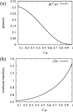
Figure 1. The initial equilibrium with the  and
and  m magnetic configuration; (a) the m/n = 0/0 component of the pressure projected on the Boozer coordinate; (b) the rotational transform of the equilibrium.
Download figure:
Standard image High-resolution imageSince LES is a numerical method, which is based on the assumption that the flow is turbulent and the nonlinear energy transfer from a large scale to a small scale can be replaced by a Smagorinsky-type (an eddy-viscosity-type) model, we should first verify that the plasma dynamics is turbulent at a nonlinear stage of time evolution. In figure 2, the pressure spectrum at the time of the nonlinear saturation is shown as a function of the poloidal wave number m for a computation of  and
and  . The plot is scattered for the toroidal wavenumber n < 20 so that we see 20 points for a single value of m. It is seen in figure 2 that the Fourier energies of the pressure are excited over a wide range of the wavenumbers, and show a tendency in which the Fourier energies may be scaled by the power of the wavenumber m, as we often see in the MHD and Hall MHD turbulence spectrum [15, 26]. In the figure, it is difficult to find reminiscent linear eigenfunctions once formed at the linear stage of the simulation. Some n = 2 coefficients have the largest values of all ns. However, it looks fully turbulent when we see the pressure fluctuation on a poloidal cross-section, being different from those observed at the linear stage (the figure is omitted), due to the strong stretching, entrainment and mixing of the pressure on a poloidal cross-section by the vortices generated originally by the unstable ballooning modes. Thus, the dominance of the n = 2 Fourier coefficients does not necessarily mean the dominance of the ballooning mode itself, but rather that of a structure which has survived the nonlinear stage.
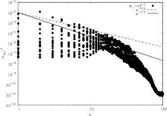
Figure 2. The energy spectrum of the pressure at the saturation time in the nonlinear single-fluid MHD simulation of the ballooning modes of LHD.
Download figure:
Standard image High-resolution imageSecond, we estimate how much the SGS terms can contribute to the mild saturation of unstable modes by making use of our earlier numerical data. While numerical results in [7] show a large collapse at the plasma core, the growth of unstable modes is mildly saturated for the same initial equilibrium when the viscosity is set higher ( in [5]). Thus, estimating how a large
  can grow in a simulation in comparison to
  provides an insight for the magnitude of
  . The time evolution of
  in equation (27) by using the numerical data in [7] is plotted in figure 3(a), and the isosurfaces of
  at the time of nonlinear saturation are shown in figure 3(b) for
  according to [16] for incompressible channel MHD turbulence. (For Hall MHD turbulence, we consider that
  can work better than
  for reproduction of the spatial structures, although it is too diffusive to reproduce the energy spectrum [18].) With respect to the importance of the parameters in the simulations,
  and the number of grid points
  in the reference simulation in [7] as well as
  and
and  have been set to the same resolution as in [5]. Note that the growth of the unstable modes in the latter computation is mildly saturated and that well-formed magnetic surfaces are recovered autonomously after saturation. The plot indicates that the truncated SGS components can play the role of a viscosity that is as high as
  to the GS (low-wavenumber) modes through nonlinear couplings. Since the maximum value of the SGS viscosity in figure 3(a) is higher than
  , it is expected that the introduction of the SGS viscosity can lower the saturation level of the instability, although it is also considered that mild saturation of the instability cannot only be achieved by the introduction of the SGS effects, because the unstable low modes can grow linearly before the SGS effects begin to work. Since the estimation of the
  is for the grid points of
  , the role of the SGS components on the GS components can be larger for a smaller number of grid points.

Figure 3. (a) The time evolution of the mean (solid) and the maximum (dotted) values of the SGS viscosity estimated from the simulation in figure 2. (b) The isosurface of  defined in equation (27) in a nonlinear simulation.
Download figure:
Standard image High-resolution image3.2. Parameter surveys on the Smagorinsky coefficients and a restriction in the SGS coefficients
Based on an assessment of the LES approach, we carry out the LESs of ballooning modes with a number of grid points  . The number of grid points is 1/4 of our earlier computations, and the time step width is also coarser. This coarse-graining in both time and space decreases the computational cost significantly. We do not carry out LESs with a smaller number of grid points (larger grid width), because our earlier studies on homogeneous Hall MHD turbulence [15, 27] show that very coarse low-pass filtering can bring about a considerable change in the nonlinear interaction of the Hall term at low wavenumbers. This simply means that solving the equations with a very coarse grid width cannot express the nonlinear dynamics of the low modes, even if we compensate for some aspects of the nonlinear interactions using the SGS models. As far as we have examined, the grid width should be as small as, or smaller than, the ion skin-depth in order to avoid significant change—unless we develop a new SGS model which can correct the change of the nonlinear interaction at low wavenumbers. (This is another way of mentioning the importance of turbulent high-wavenumber components to unstable low modes.) Thus we set the number of grid points
  in this paper for the Hall parameter
  (the ion skin-depth is comparable to the grid width) or to
  (the ion skin-depth is larger than the grid width).
In figures 4 and 5, a typical example of an LES result is shown by use of the parameters  and
and  (run LES41). See table 1 for the typical LESs and parameters used for each of the runs. In figure 4(a), the isosurfaces of the pressure and the streamlines at the end of the linear stage of an LES, magnified around a poloidal cross-section, are shown. The streamlines show that flow is generated in the poloidal (binormal) direction. Since the poloidal flow does not appear in the single-fluid MHD simulations and appears as the result of the introduction of the two-fluid effect, it is considered to have been generated by the diamagnetic effect. Because of the flow in the poloidal direction, we can observe that the pressure profile is elongated in the poloidal direction, causing thermal mixing and homogenization in the direction of a fully nonlinear stage (the figure is omitted). In figure 4(b), the isosurfaces of the pressure, magnetic field lines (thick tubes) and streamlines (thin tubes) at a nonlinear stage are shown for the fully torus geometry. The streamlines are spirally elongated along the magnetic field lines in some regions, and drift in the poloidal direction, forming a turbulent mixed drift-vortex structure in some other regions. In this sense, plasma motion is turbulent in some regions while a simple vortex motion along the magnetic field lines can dominate in some others.

Figure 4. (a) The isosurfaces of the pressure and the streamlines at the end of the linear stage of an LES, magnified around a poloidal cross-section. (b) The isosurfaces of the pressure, magnetic field lines (thick tubes) and streamlines (thin tubes) in the fully saturated state of an LES (fully torus image). The sampling points of the streamlines are more localized near the  rational surface than those in (a).
Download figure:
Standard image High-resolution image
Figure 5. The time evolution of the energy of each toroidal mode n of (a) parallel and (b) normal components of the velocity obtained by an LES of  .
.
Download figure:
Standard image High-resolution imageTable 1. The parameter sets studied in this paper.
| Run-name |  |
 |
SGS model |  |
 |
 |
Low-pass filtera |
|---|---|---|---|---|---|---|---|
| LES41 | 10−1 | 0.0125 |  |
0.046 | 0.046 | 0.046 | off |
| LES42 | 10−1 | 0.0125 |  |
0.46 | 0.46 | 0.46 | off |
| LES45 | 10−1 | 0.0125 |  |
0.46 | 0.46 | 0.046 | off |
| LES49 | 1 | 0.0125 |  |
0.046 | 0.046 | 0.046 | off |
| LES50 | 1 | 0.0125 |  |
0.46 | 0.46 | 0.46 | off |
| LES118 | 10−1 | 0.05 |  |
0.46 | 0.92 | 0.46 | off |
| LES119 | 10−1 | 0.05 |  |
0.46 | 1.38 | 0.46 | off |
| LES120 | 10−1 | 0.05 |  |
0.23 | 1.38 | 0.46 | off |
| LES121 | 10−1 | 0.05 |  |
0.092 | 1.38 | 0.46 | off |
| LES122 | 10−1 | 0.05 |  |
0.46 | 0.92 | 0.46 | on |
| LES123 | 10−1 | 0.05 |  |
0.46 | 1.38 | 0.46 | on |
| LES124 | 10−1 | 0.05 |  |
0.23 | 1.38 | 0.46 | on |
| LES125 | 10−1 | 0.05 |  |
0.092 | 1.38 | 0.46 | on |
| LES126 | 10−1 | 0.05 |  |
0.46 | 0.92 | 0.92 | off |
| LES127 | 10−1 | 0.05 |  |
0.46 | 1.38 | 0.92 | off |
| LES128 | 10−1 | 0.05 |  |
0.23 | 1.38 | 0.92 | off |
| LES129 | 10−1 | 0.05 |  |
0.092 | 1.38 | 0.92 | off |
| LES130 | 10−1 | 0.05 |  |
0.46 | 0.92 | 0.92 | on |
| LES131 | 10−1 | 0.05 |  |
0.46 | 1.38 | 0.92 | on |
| LES132 | 10−1 | 0.05 |  |
0.23 | 1.38 | 0.92 | on |
| LES133 | 10−1 | 0.05 |  |
0.092 | 1.38 | 0.92 | on |
aBesides the low-pass filter for the LES, another low-pass filter of the fourth order explicit formulation presented in [28] is operated on the fluctuation components of the density, momentum and pressure fields at the end of the fourth stage of the Runge–Kutta marching step in order to remove high-wavenumber components when it is 'on'.
In figure 5, the time evolution of the Fourier energy of each toroidal mode n of (a) parallel and (b) normal components of the velocity obtained by the LES is shown. In figure 5 the Fourier energies grow exponentially at the beginning of the time evolution. The growth rate is largest in n = 1 due to a large  . Furthermore, the parallel component is much larger than the normal component, being similar to our single-fluid MHD results in [6, 7]. These results show that our LES reproduces a qualitative nature in the ballooning modes of LHD with a higher numerical resolution in [7]. We have also compared the results with a simulation that does not have the SGS terms. Although a simulation which is carried out without the SGS terms and without a sufficient resolution cannot go beyond nonlinear saturation, it can reproduce the beginning of the linear regime of low modes. So far as we have compared the growth rates between the two runs, LES41, and the run without the SGS terms, the growth rates of the low modes differ by only a few percent or less (the figure is omitted). This is quite natural, because the SGS models are essentially nonlinear, so that the SGS terms begin to work in the nonlinear phase, and do not contaminate the linear regime. Note here that the plasma dynamics can be contaminated by the SGS terms when the SGS coefficients are too large, and we must restrict ourselves so that the SGS coefficients are not too large. Since the SGS coefficient is given by equation (27), making
  and
and  ten times larger simultaneously can be translated as
  to
to  . In other words, the filter length
  is effectively doubled by enlarging
  and
and  ten times, and the unstable mode resolved in the grid scale is halved. As a consequence, it should appear in an LES as the energy loss from the GS to SGS (lower GS energy in comparison to an LES with smaller Smagorinsky coefficients.) We intend to study the low-mode—
 in the coarsest case and
  for a more preferable case—without the contamination of the SGS terms. In [16],
  is used based on their turbulence theory. Here, we should not forget that the applicability of the LES approach is based on our earlier research in which the forward energy transfer becomes dominant at scales smaller than the ion skin depth. This also restricts the values of
  and
and  , or
, or  equivalently. This is the origin of the SGS coefficients for LES41, although
  can work better than
  for reproduction of the spatial structures in turbulence with the Hall effects [5]. Supposing the resolution of
  in the coarsest case, we consider
  to be preferable, and
  adopted in some runs can be quite marginal, although there is no clear estimation of
  , because this is the first case to introduce the SGS model for our extended MHD system. This is the reason why we have restricted the Smagorinsky coefficients in the range seen in table 1. Since we carry out LESs which aim to solve low modes with the help of SGS effects, we should verify how low modes are solved in the linear stage of a simulation. The pressure and velocity Fourier coefficients in a computation in [7] (the number of grid points
  and the parameters
  ) agree well with those of the linear eigenfunctions at each m and n for
  . We make use of the results there as reference data. Since the numerical resolution in the radial and poloidal directions in the LESs here is half that of the reference data, we can expect the resolution of the Fourier coefficients of n < 6 for the linear phase of our LESs.
In figure 6, the radial profiles of the Fourier coefficients of the pressure for (a) n = 1 and (b) n = 3 with some poloidal wavenumber m in the run LES41 are plotted as a function of the initial magnetic flux function  . A combination of the wavenumbers m and n is provided for
  because the pressure gradient is steepest there. The radial profile is plotted at a time when the time evolution shifts from the linear stage (exponential growth of the Fourier energy) to the nonlinear stage. It is seen in figure 6(a) that the Fourier coefficients at
  have the largest amplitude at that time, and the Fourier coefficients peak at
  where the pressure gradient is steepest. (The vertical axis in the plots is essentially arbitrary in the sense that the Fourier coefficients form a linear eigenfunction of the unstable modes for each n.) In figure 6(b), the Fourier coefficient of m/n = −5/3—not of m/n = −6/3—has the largest amplitude and its peak appears at
  . The dominance of m/n = −5/3 for the n = 3 mode, in spite of the large pressure gradient at
  , is a consequence of the coupling with the m/n = 1/0 coefficient, which is a residue from obtaining the initial equilibrium by using the HINT code [19]. (The influence of m/n = 1/0 has been already reported in [6].) Since it is the result coming from the initial equilibrium, we consider the linear nature to be well resolved for n = 3 too. Fourier coefficients in LES41 for
  do not necessarily form a clear radial profile, partially because the high parallel heat conductivity
  tends to suppress the formation of the Fourier coefficients to be like linear eigenfunctions as n becomes larger (a computation with
  has been used for studying the radial profile in [7]), and partially because of the influence of the SGS terms.
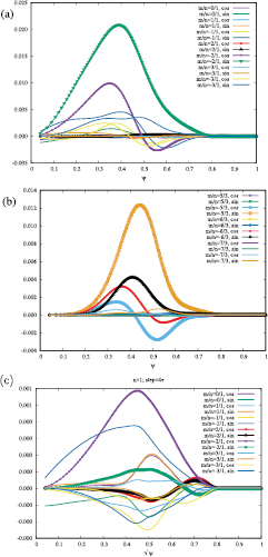
Figure 6. The radial profiles of the pressure Fourier coefficients for (a) n = 1 in LES41, (b) n = 3 in LES41 and (c) n = 1 in LES42. The time of the snapshots is chosen so that the radial profiles of the Fourier coefficients are well formed after the initial transients. The vertical axis is essentially arbitrary in the sense that the Fourier coefficients form a linear eigenfunction of the unstable modes for each n.
Download figure:
Standard image High-resolution imageIn figure 6(c), the radial profile of the n = 1 Fourier coefficients in LES42 is plotted at the same time as (a) and (b). The outline of the radial profile is similar to that in figure 6(a), specifically for the main harmonic m/n = −2/1. However, we may find that the main harmonic m/n = −2/1 is slightly different between figures 6(a) and (c), at  . The harmonic in figure 6(c) changes more slowly than that in (a). Although figure 6(c) is for the plot of the linear stage in LES42, it might come from the SGS coefficients in LES42, especially from those for the heat conduction
  , which are larger than those in LES41 by ten times or more. In other words, adopting SGS coefficients that are too large can contaminate the linear stage of unstable modes, even though the SGS models in equations (28)–(30) are provided so as not to contaminate the linear stage. Based on the parameter surveys over a wide range of the SGS coefficients
  ,
,  and
and  , we restrict our computational works here to those shown in table 1 so that the nonlinearity in the SGS terms does not contaminate the linear evolution too much.
In figure 7, the radial profile of the m/n = 0/0 component of the pressure is plotted at some moments from the initial to the saturation time. Figure 7(a) is for an LES of (a)  , and figure 7(b) is for an LES of (b)
  =
=  =
=  . Both of the two runs give nonlinear saturation even though the numerical resolution is not very fine. (The saturated state is not perfectly in a steady state because of the absence of the source and sinks. However, the profiles are in a slowly decaying state after the saturation of the energy growth and a drastic change in the profiles is not observed in the phase.) Though the SGS viscosity becomes high in the turbulent regions of the LESs, as we have estimated in the previous section, the plasma core in figure 7(a) finally collapses. The collapse is a consequence of the growth of the low modes without artificial damping by a large viscosity. The growth is sharply different from that of earlier simulations with
  in [5], in which the growth rate of the linear low modes is considerably lowered by the viscosity. This shows that a high and uniform viscosity should not be adopted for the study of instability, and that the SGS viscosity which represents the energy transfer from the GS to the SGS components should be used instead. While figure 7(a) gives a deteriorated profile of P00, the set of SGS coefficients in (b) gives a better result than (a).

Figure 7. The mean pressure profile  in two LESs, (a) LES41 (
 ) and (b) LES42 (
 ).
).
Download figure:
Standard image High-resolution imageRecall here that flattening of the total pressure is not observed in experiments [17]. In other words, we consider the baseline as keeping a peaked pressure at the core ( ). Since figure 7(b) allows total collapse of the pressure to be avoided, meaning a low but finite peak is kept at the center of the core, the LES approach is considered to be able to reasonably compensate for a lack of numerical resolution in a simulation and enable a smaller, quicker numerical simulation. However, we must keep in mind that the SGS coefficients should be calibrated more carefully, so that the SGS models represent the influence of turbulent fluctuation on linear low modes, in accordance with simulations with a higher resolution as well as experiments. Also note that the computational cost is about 1/32 or less than the earlier computations reported in [10], in which the number of grid points is
  and a strong numerical filter is applied to eliminate very fine (both in time and space) motion.
3.3. Saturated pressure profile
Now we carry out the LESs of the ballooning modes to see how the SGS coefficients can influence the saturated profile of the pressure, for SGS coefficients that are larger than those in LES41 and LES42. Although appropriate values of the SGS coefficients should be determined through calibration with large computations of very high resolution, without SGS models as well as with many experimental results, the parameter survey over a wide range of SGS coefficients can clarify the possible contributions of the SGS terms to the saturation profile of the pressure and dynamics of the low modes.
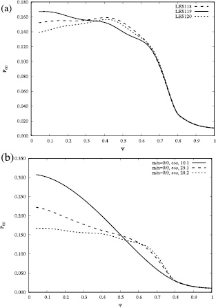
In figure 8(a), saturated P00 in runs LES118, LES119 and LES120 are plotted as a function of  . While P00 in LES118 and LES120 are hollow at the plasma core, P00 in LES119 peaks at
  . The pressure deformation associated with advection is considered to be relatively suppressed in LES119 because
  in LES119 is larger than that in LES118 and LES120. This observation means that turbulent fluctuation on the SGS scale can interact with unstable modes and suppress the pressure deformation through the nonlinear interaction. In figure 8(b), the change of P00 in time in the run LES119 is plotted. As we have already seen for other parameter sets, the P00 profile deteriorates as the unstable modes grow. However, at the final stage of the saturation, the plasma core avoids becoming hollow. This suggests that turbulent fluctuations, the roles of which are represented through SGS terms, can work to terminate the final crash by strong nonlinear couplings, although it is difficult for them to suppress the growth of unstable low modes completely, because unstable low modes can grow to sufficiently large amplitudes before turbulent fluctuation terminates the growth of the low modes.
Figure 8. (a) A comparison of the radial profile of P00 as a function of  for the runs LES118, LES119 and LES120. (b) Change of the radial profile P00 in time in the run LES119.
Download figure:
Standard image High-resolution image
Finally, it is mentioned that some parameters have been examined but not presented in this paper. For example, we have examined the influence of an additional low-pass filter on the strong stabilization of the computations. A distinction of the adoption of the additional low-pass filter is indicated by 'on'/'off' in the table. It is noted here that the introduction of the low-pass filter does not affect numerical results significantly.
4. Discussion and concluding remarks
We have introduced the concept of the LES for a simulation study of the mild saturation of the unstable ballooning modes of a heliotron device, and developed SGS models that are suitable for two-fluid MHD equations. Fully 3D LESs of two-fluid MHD equations are carried out for the  m unstable magnetic configuration of LHD. Our LESs achieve the nonlinear saturation of the ballooning modes by a coarse numerical resolution without contaminating the linear growth of the unstable modes up to moderate wave number. However, the plasma pressure is reduced considerably in the LESs, suggesting that neither the generation of spontaneous diamagnetic drift nor the SGS components are sufficient to suppress the growth of the ballooning modes. Since the initial equilibrium in the LESs reported here has neither finite flow nor flow shear, this disagreement might be attributed to the finite flow shear effects generated through a rise in the β-value, rather than the two-fluid and SGS models.
With respect to the diamagnetic drift and the flow shear, we consider that the route of the plasma dynamics to the β-value might be important. The  is one of the most unstable parameter ranges for this magnetic configuration. In the course of the β value increasing up to
  , the plasma can come to a less unstable state, keeping the generation of diamagnetic flows. As a consequence, plasma can have a stronger diamagnetic flow than that generated spontaneously by the instability for the
  equilibrium. A study on such a strong diamagnetic flow and/or flow shears should be one of our next studies. It is emphasized here again that a strong flow shear together with gyro-viscous effects often excites very small scales, and thus knowing the influence of the SGS components on the subject can be essential. The development of the SGS model for two-fluid MHD equations enables numerical simulations of the growth of unstable modes with such a flow shear. When a strong flow shear excites very small scales, small-scale flows are assumed to transit to a turbulent state, and cause further energy transfer from large to small scales. Turbulence effects can influence large scales through the Smagorinsky model, even though the small scale components are filtered out, assuming the small-scale flows cascade toward smaller scales. One of the most important points for such a case is how large the Smagorinsky coefficients should be. We consider that we are able to calibrate the Smagorinsky coefficients by carrying out a closer comparison of our LESs to either experiments or numerical simulations without the SGS models, but with a very high numerical resolution. We may also consider adjusting the Smagorinsky coefficients autonomously in accordance with the excitation of the small scales, for example by the dynamic Smagorinsky model. (See the text by Garnier et al in the reference list therein for the dynamic Smagorinsky model.)
While sufficient stabilization of the unstable modes has not been obtained through the parameter survey on the SGS coefficients, the change in the saturated pressure profile depending on the SGS coefficients suggests that the unresolved scales in a two-fluid MHD simulation can contribute considerably to the retention of plasma core pressure. This suggests, in the context of understanding the experimental results, that the interaction of turbulent fluctuation with the instability can modify the plasma dynamics considerably. Appropriate values of the SGS coefficients will be determined through calibration of the coefficients to larger computations with a very high resolution and without the SGS models, and to many experimental results. Furthermore, though we have only compared the pressure profile, the poloidal flow is also important because of the existence of flow shears mentioned above. From this point of view, a quantitative comparison of our LES results with the experiments should also be carried out. The calibration results will be reported elsewhere.
We have not studied detailed structures observed through the magnetic field lines, such as magnetic stochasticity. Magnetic stochasticity on a small scale should be included in the SGS terms. We consider that the degree of magnetic stochasticity in the present model is not sensitive to the SGS dissipation coefficients. A considerable part of the magnetic stochasticity can appear associated with the growth of low modes which have wide eigenfunctions. On the other hand, the influence of high modes, which are modeled through the SGS terms, is restricted to a narrower region than the lower modes, with smaller Fourier amplitudes being included in the SGS model easily. As for magnetic field induction, we may need a more complicated model than the traditional Smagorinsky-type model in order to take the dispersive nature of the Hall term into account more accurately. Such an advanced model has now been developed and tested for homogeneous Hall MHD turbulence. However, for studies of low-pressure-driven modes in a helical device, it appears that the effect of the dispersive waves associated with the Hall term are not very clear, and a higher priority should be put on the study of flow effects.
Finally, the LES approach also enables a drastic reduction in the computational cost and a better representation of dynamics in two-fluid MHD simulations of strong ballooning modes without damping the modes excessively, and thus provides much easier access to the study of the saturation mechanism of unstable modes in a heliotron device. We believe this will help carry out many case studies on instability and two-fluid phenomena in a heliotron device.
This research was partially supported by JSPS KAKENHI, grant number 23540583 and MEXT KAKENHI grant number 15H02218, Japan. This research was also partially supported by the Joint Institute for Fusion Theory (JIFT) program in the US-Japan collaboration for fusion studies. The numerical simulations were performed on a FUJITSU FX100 supercomputer Plasma Simulator at NIFS with the support and under the auspices of the NIFS Collaboration Research Program (NIFS15KNSS053, NIFS15KNTS038). Some of the simulations were also performed on the FX100 of Nagoya University based on the HPC project of Nagoya University, and the HELIOS supercomputer system at the Computational Simulation Centre of International Fusion Energy Research Centre (IFERC-CSC), Aomori, Japan.