

Abstract
Current time domain facilities are finding several hundreds of transient astronomical events a year. The discovery rate is expected to increase in the future as soon as new surveys such as the Zwicky Transient Facility (ZTF) and the Large Synoptic Sky Survey (LSST) come online. Presently, the rate at which transients are classified is approximately one order or magnitude lower than the discovery rate, leading to an increasing "follow-up drought". Existing telescopes with moderate aperture can help address this deficit when equipped with spectrographs optimized for spectral classification. Here, we provide an overview of the design, operations and first results of the Spectral Energy Distribution Machine (SEDM), operating on the Palomar 60-inch telescope (P60). The instrument is optimized for classification and high observing efficiency. It combines a low-resolution (R ∼ 100) integral field unit (IFU) spectrograph with "Rainbow Camera" (RC), a multi-band field acquisition camera which also serves as multi-band (ugri) photometer. The SEDM was commissioned during the operation of the intermediate Palomar Transient Factory (iPTF) and has already lived up to its promise. The success of the SEDM demonstrates the value of spectrographs optimized for spectral classification.
Export citation and abstract BibTeX RIS
1. Introduction
It is now widely agreed that time domain astronomy (TDA)—the study of transients, variables, and moving objects—is one of the frontier fields of this decade (NationalResearchCouncil 2010). The first systematic time domain astronomical program was initiated by Fritz Zwicky with an 18-inch Schmidt telescope (commissioned in 1936) survey sited at the Palomar Observatory. Over 38 years, the program allowed the discovery of 380 supernovae (SNe), with an average rate of 10 per year. As can be seen in Figure 1, the annual haul of SNe increased and remained steady at 30 per year well up into the 1990s, routinely crossing the 100 mark only by the new millennium. Over this period, the major advances in the field were the recognition of supernova in the elemental build up of the universe and the use of type Ia supernovae for cosmography.
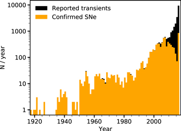
Figure 1. Transient events reported per year (black) and confirmed supernovae (orange) per year between 1916 and 2017. Source: http://www.rochesterastronomy.org. The discoveries may contain a fraction of galactic transients or extreme variability in AGN.
Download figure:
Standard image High-resolution imageThe ultimate rise of TDA has been driven entirely by technological progress in sensors and computing. During the last two decades, more than a dozen optical TDA surveys arose, e.g., the Catalina Sky Survey (Drake et al. 2009), Pan-STARRS-1 (Kaiser et al. 2002), the (intermediate) Palomar Transient Factory (iPTF; Rau et al. 2009), ASASSN (Shappee et al. 2014), and ATLAS (Tonry 2011). As a result of these surveys, the supernova discovery rate has increased dramatically and the current annual rate of classified supernovae is over 1000.10 The large sample size has resulted not only in the discovery of new classes of supernovae (e.g., super-luminous supernovae), but also of new sub-classes of extragalactic explosions (e.g., intermediate luminosity optical transients, luminous red novae, and calcium-rich supernovae). Separately, new types of eruptive variables (e.g., extreme variability in active galactic nuclei (AGN)) and cataclysmic explosions, e.g., tidal disruption events (TDEs) are now routinely found. New upcoming surveys such as the Zwicky Transient Facility (ZTF; Bellm 2014), BlackGEM11 , and the Large Synoptic Sky Survey (LSST; Ivezić et al. 2008) will push the discovery rate even higher, discovering up to hundreds of new supernovae every night.
We expect the discovery rate of supernovae to continue a dramatic growth, thanks to these ongoing and planned surveys. However, identifying supernovae candidates is merely the first step. Only with the second step—spectral classification—is the discovery process completed. However, spectroscopy requires follow-up observations in most instances on telescopes with apertures larger than that of the discovery telescope. As shown in Figure 1, the growing gap between the rate at which transients are identified and classified is truly an "elephant in the room."
Traditionally, low-resolution spectroscopy meant a spectral resolution of  . Fortunately, spectral classification of supernovae and TDEs, with their large expansion velocities,
  can be done with lower spectral resolution.
Next, robotic spectroscopy would be very helpful, given the increasing discovery rate of transients. These two considerations have led to "intermediate resolution" ( ) spectrographs on robotic telescopes: the low-resolution cross-dispersed spectrograph (FLOYDS; Brown et al. 2013) operating on two 2-m robotic telescopes, part of the network Las Cumbres Observatory Global Telescope (LCOGT) and SPectrograph for Rapid Acquisition of Transients (SPRAT; Piascik et al. 2014), mounted at the 2-m robotic Liverpool telescope in La Palma, Spain.
One of the challenges for robotic spectroscopy is in placing the target precisely on the narrow (1–2'') slit. This usually results in an iterative target acquisition approach, where the failure rate may increase due to complex host-galaxy environment or non-ideal observing conditions. This problem can be solved by using an integral field unit (IFU) spectrograph with a reasonably large field of view (FOV; say 15'' or larger). This concept was first explored with the SuperNova Integral Field Spectrograph (SNIFS; Lantz et al. 2004), a medium-low integral field spectrograph dedicated to the observation of supernovae for cosmology. Although with a smaller FOV (6 × 6''), SNIFS proved that this approach, apart from the ease of target acquisition, has the additional advantage of the study of the supernova environment.
Thus, a major step forward in filling the gap of transient follow-up can be made by deploying a low-resolution, robotically controlled IFU spectrograph with  and an FOV of, say, ≈30'' square on a dedicated 1 m class telescope with sufficient throughput to achieve a signal-to-noise ratio (S/N) of 5 for a 20.5 r-band magnitude transient (the faint end of current TDA surveys) with an exposure time of 3600 s. The design for just such instrument was conceived in 2009 as a resource for spectroscopic follow-up of transients discovered by PTF. Here, we present an overview of "Spectral Energy Distribution Machine" (SEDM) optimized for rapid classification spectroscopy. The SEDM has been operating at the Palomar 60-inch telescope (P60) since 2016 April 27. In 2016 August, it became the primary instrument on this telescope.
The paper is organized as following. Section 2 provides an overview of the instrument design and main characteristics. Section 3 describes the daily operations and data flow. The photometric and spectroscopic reduction pipelines are explained in Section 4. We provide an overview of the performance in Section 5, and a summary of the first scientific results of SEDM in 6. Finally, Section 7 offers a discussion of the next steps for the SEDM project and the implications for future transient searches at optical wavelengths.
2. Instrument Overview
The SEDM is currently the sole instrument deployed on the robotically controlled Palomar 60-inch telescope (P60). The telescope optics are Ritchey-Chrétien, so that both primary and secondary mirrors have hyperbolic reflecting surfaces. This allows for a wider FOV within a compact design: the tube of the telescope measures 150 inches (3.8 m) long. An 18-inch (45.7 cm) central hole in the primary mirror allows starlight to reach the Cassegrain focus (f/8.75) with a 525-inch (13.3 m) focal length. The telescope was roboticized in 2004 and single-purposed for imaging photometry, in particular following gamma-ray burst (GRB) afterglows (Cenko et al. 2006). In 2016 August, the GRB imaging photometer was replaced by SEDM as the primary instrument at the Cassegrain focus of P60.
The SEDM instrument is composed of two main channels: the Rainbow Camera (RC) and the Integral-Field Unit (IFU), mounted in a T-shaped layout (see Figure 2). The optics and cameras are protected by an external cover, designed as a sealed container to minimize light and dust contamination. Overall, the instrument is of a compact size, of 1.0 × 0.6 m. The total weight, including electronics, is of ∼140 kg.

Figure 2. Overview of SEDM instrument layout. The light path from the Cassegrain focus is shown with a red arrow. The photometric instrument (RC) gathers the direct light, and is located at the top center. The light for the IFU is initially redirected toward the mirror on the left side of the picture, and is reflected into the MLA barrel (labeled Lenslet). The light from each microlens is then dispersed by the triple prism system, held by the brown fixture in the center, and then focused by the camera optics (labeled IFU Barrel) onto the IFU Camera.
Download figure:
Standard image High-resolution imageThe optical path of the instrument is designed so that most of the light from the Cassegrain focus is directed toward the photometric instrument, the RC. The light for the IFU is captured by a pickoff prism that is mounted at the center of the four filter holders for the RC, close to the telescope focal plane.
Both the IFU and the RC have relay optics that allow the images to come to focus at their respective CCD detectors, as well as an independent focus mechanisms to ensure that the RC and the IFU channels are parfocal. The RC is focused by adjusting the position of the movable telescope secondary mirror to achieve the minimum FWHM of star images. The spectrograph is focused using movable camera optics to achieve the minimum FWHM of arc-lamp lines. The IFU is then focused by moving one of the expander lenses to achieve the minimum FWHM of a bright star on the IFU camera, thus ensuring the RC and IFU cameras are parfocal.
The SEDM uses two identical Princeton Instruments, Pixis 2048B and eXelon CCDs, each having an array of 2048 × 2048 13.5 μm pixels. The CCD windows are anti-reflection coated to improve overall response. The cameras have thermoelectric coolers to keep the detectors at a temperature of −55°C. The excess heat is removed via a glycol cooling system attached to a chiller. A summary of the specifications for the detectors is shown in Table 1.
Table 1. Specifications for the SEDM Detectors
| Detector feature | Description |
|---|---|
| Detector size | 2048 × 2048 pix |
| Pixel size | 13.5 μm |
| Read noise (slow) | 5 e−/pix |
| Read noise (fast) | 22 e−/pix |
| Read time (fast) | 5 s |
| Read time (slow) | 40 s |
| Gain | 1.8 e−/ADU |
| Non-linearity | 45,000 ADU |
| Saturation | 55,000 ADU |
Download table as: ASCIITypeset image
2.1. Rainbow Camera
The RC is used for guiding, calibration, target acquisition, and science imaging. The 13 × 13 arcmin FOV is split into four quadrants, one for each filter:  ,
,  ,
,  , and
, and  . Because part of the field is obscured by the filter holder, only
  arcmin field is available for imaging the target with each filter. To obtain an exposure with a different filter, the telescope is offset to center the target in a new quadrant. A raw SEDM image is shown in Figure 3, where the Crab Nebula can be seen in the
  panel. The blue rectangle shows the position of the IFU pickoff prism.
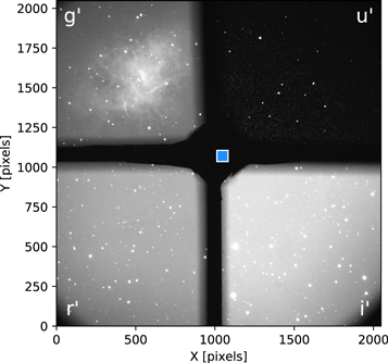
Figure 3. Raw RC image. The Crab Nebula can be seen in the upper left corner, being imaged through the g-band filter. The different level of background for each filter is a function of sky color and filter-detector throughput. The u-band has the lowest throughput. The blue square indicates which part of the field is directed to the IFU by the pickoff prism.
Download figure:
Standard image High-resolution imageThe RC uses Astrodon12
generation 2 filters. Their transmittances are shown in Figure 4, along with the predicted quantum efficiency of the CCD at the nominal operating temperature of  C. The specifications for each filter, pixel size, and single filter FOV are shown in the upper part of Table 2.

Figure 4. Astrodon generation 2 filters transmittance used for the RC. The CCD quantum efficiency at the nominal operating temperature ( C) is shown with a dashed line.
Download figure:
Standard image High-resolution imageTable 2. Instrument Specifications for the RC and IFU
| RC Specification | Descriptions |
|---|---|
| FOV (single filter) | 6.0 × 6.0 arcmin |
| Pixel scale | 0.394'' |

|
355 nm |

|
477 nm |

|
623 nm |

|
762 nm |

|
67 nm |

|
148 nm |

|
134 nm |

|
170 nm |
| IFU Specification | Description |
| FOV | 28 × 28'' |
| Pixel size | 0.125'' |
| MLA size (spaxels) | 45 × 52 |
| Single microlens diameter | 0.75'' |
| R | ∼100 |
| Dispersion | 17.4–35 Å/pix |
Download table as: ASCIITypeset image
2.2. Integral Field Unit
The SEDM IFU consists of a microlens array (MLA) covering 28 × 28'' with 45 × 52 hexagonal microlenses that project their beams through a triple prism that produces a near constant spectral resolution of  .
.
A pickoff prism intercepts a field of size 28 × 28'' from the center of the f/8.75 P60 beam. The pickoff location minimizes the field lost by the RC. The prism directs the light through an expander lens to obtain an appropriate image scale for the MLA. Then, the light path is folded by a flat mirror, and directed through a field-flattening lens onto the MLA. The MLA breaks up the field into an array of 2340 hexagonal pupil images of 0.75'' in diameter, which are sent through a six-element collimator onto the dispersing triple prism. The triple prism design ensures that the spectroscopic resolution, defined as  , is close to a constant value of
  . The dispersed pupil images are then focused by a five-element camera through a CCD window that is multi-coated for high transmission. As an example, Figure 5 shows the IFU image of Saturn as directly projected on the detector. A summary of the specifications of the instrument are shown in lower part of Table 2.

Figure 5. Raw negative IFU image of Saturn. The exposure time is 1 s. The size of the IFU covers 28 × 28''.
Download figure:
Standard image High-resolution image3. Operations and Data Flow
The SEDM observing system relies on several hardware and software components, shown in Figure 6. These resources are distributed between the Palomar Observatory and the Caltech campus. In this section, we provide a description of the operations for the main software modules for SEDM.
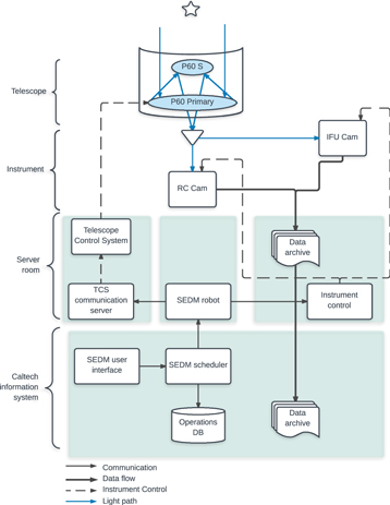
Figure 6. Schematic representation of the SEDM hardware and software modules. A web user interface allows observers to create observation requests, which are scheduled for the night. The robot uses the schedule to communicate with the telescope and the instrument to carry out the exposures and send the data from Palomar to the Caltech data archive. The green background boxes indicate a dedicated computer and the white boxes show the functions that are operating within the given computer.
Download figure:
Standard image High-resolution image3.1. SEDM Startup
What follows below is a description of the flow of activities for a typical day. At 4:00 PM PST, the Palomar crew release the P60 to the astronomical operations group. The master program then initializes the main software module controlling the instrument (the SEDM robot) and also creates a simulated schedule for the night. Diagnostic checks are undertaken to ensure that the various sub-systems (telescope; dome; IFU and RC; data processing computer; and archival computer) are operating. Should a failure be detected then an automated warning is issued. On-site personnel then have about 1 to 2 hours to diagnose and fix the problem.
Once all diagnostic checks are successful, the automation script begins a series of bias, arc-lamp, and dome-flat observations using the IFU camera. For the RC camera, in addition to the above, a set of twilight flats are undertaken (provided the weather conditions permit opening of the dome).
Just before nautical twilight, the system runs a focus loop using the secondary stage on the P60. A bright star is selected from the Smithsonian Astrophysical Observatory (SAO) star catalog according to visibility and airmass constraints. The focus for the RC is obtained from a set of short exposures on the target. The last best focus position is used as an initial position, and the stage of the secondary mirror moves five steps on each side, with an increment of 0.25 mm. A two degree polynomial is fit to the FWHM of the images in all four filters to interpolate the new best focus position. To maintain the parfocality of the RC and the IFU, a similar process is followed for finding the focus of the IFU. In this case, we fit FWHM corresponding to the point spread function (PSF) of the image obtained by collapsing 3D IFU cube along the wavelength axis.
At the beginning of nautical twilight, the robot finishes the initial calibration phase by taking a standard star observation.
3.2. Acquisition Process
The acquisition process for IFU science targets is shown in Figure 7. For each object, a single 10–20 s acquisition exposure is taken with the RC. The resulting image is then analyzed using an astrometry fitting program to obtain the true pointing of the telescope. Typically, this step takes 20–30 s depending on the field. The robot uses this information to apply a small corrective offset to the telescope, so that the target falls in the center of the FOV of the IFU.
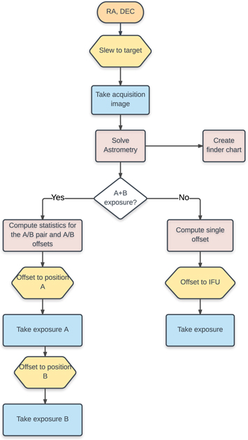
Figure 7. Acquisition process followed by the robot for science targets. The steps performed by the telescope are encoded in yellow, whereas the instrument actions are shown in blue. In red, we show the steps executed by the software acquisition modules.
Download figure:
Standard image High-resolution imageFor bright targets (<16.5 mag) only one exposure is undertaken (hereafter, an A exposure). For stars fainter than this magnitude, two exposures with identical exposure time, but with an angular offset, are undertaken (an A/B exposure). The paired images allow for a simple and robust subtraction of the background. In the case of an A/B exposure, the acquisition image is used to analyze the statistical properties of the background where the B exposure, relative to A, is going to be placed. The goal is to choose the emptiest location for the object to land in the corresponding exposure, so that a simple subtraction operation will result in efficient removal of the sky. The acquisition images are also used to create finder charts for the objects. These charts can be used during the IFU data reduction. As soon as the last exposure is complete, the robot requests the slew of the telescope to the next field, to maximize the on-sky efficiency.
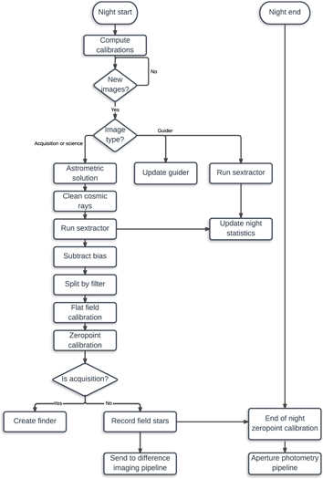
Figure 8. Data flow for the nightly data reduction pipeline. The beginning-of-night trigger activates the on-the-fly data reduction and sends the images to the difference imaging pipeline. The end-of-night trigger starts the final zeropoint calibration using all the data taken during the night, and concludes with the photometric data reduction process using the aperture photometry pipeline.
Download figure:
Standard image High-resolution imageUnder normal circumstances, the system operates autonomously through the night. The astronomical observations end with flat-field exposures undertaken at morning nautical twilight. The telescope is then stowed and a summary email of the night's observations is sent out.
Errors that occur during the night are handled and logged by the automation script. In the event of an unrecoverable error, the system is programmed to stow the telescope, close the dome, and send out an email and text alert indicating the problem.
3.3. SEDM Observatory Control System
The SEDM Observatory Control System (SOCS) is a custom-built python code designed to integrate hardware components, scheduling and processing software into one program. The python module incorporates six sub-packages that provide access to various components. By compartmentalizing these functions, the system can be easily modified and expanded in the future. The functions carried out by the packages are described below.
- Camera. This package handles communications with the cameras. Communication with these cameras are established via fiber to USB connection and a custom python package that allows the setting of various camera parameters (exposure time, gain, read-out speed amplifier, and shutter). The drivers for these cameras are currently configured for Windows, so that they run on a separate machine. The SOCS script communicates with this Windows machine via a TCP/IP socket connection.
- Observatory. This package contains scripts to handle all the physical components—telescope, dome, and arc lamps—of the observatory. Communications with the telescope and dome systems occur via a TCP/IP socket connection to the telescope control system (TCS). The arc-lamps are controlled via a network power switch.
- Sky. This package contains scripts for calculating the observing times for the target list for the night, as well as special classes of targets (e.g., GRB). Observing times are calculated using the pyephem package. A custom python class was written to create target objects. These objects contain all the metadata for each requested science target observation. This information includes the object's RA, Dec, observing constraints, and history of the observations already taken. Targets are complied from a SQL database which gets updated in real time as the observations take place.
- Scheduler. All targets are assigned a numerical priority number typically ranging from 1–5. The scheduling module then rearranges targets based on input constraints for observing cadence, Moon separation, Moon illumination, and airmass. A printout of the observing plan for the night is then made. For the rest of the night, any new targets assigned in real time into the queue will trigger the rescheduling of the night's plan.
- Sanity. The sanity package serves to make sure the telescope and cameras are all functioning properly and to prevent any actions that may cause damage to the equipment. Examples include ensuring a science target is not below the horizon limit, that the telescope will not track into a limit during a long exposure, and checking that the cameras are cooled. In addition, the sanity package also contains the error handling routines.
- Utilities. This package contains tools that help with the normal operations of the robot. These tools include FITS header management, World Coordinate System (WCS) solving, extracting best focus, and picking the best orientation for A/B pair observations for the IFU.
3.4. Guider
The tracking/guider code for the SEDM is written in python and uses Telnet to communicate with the P60 telescope guider, automatically issuing adjustments when the telescope drifts from its target. The code is stand-alone and uses only standard python packages (with the exception of telnetlib, used for communication). As such, it can be readily adapted for other uses.
The order of operations are as follows. First, a telnet connection is established with the telescope guider via hard-coded network parameters in the main configuration file. The program then continually searches for new images in the instrument's data directory, downloading them when available. Once an image is downloaded, the header is checked to see if any intentional moves or target changes have occurred. If a target change or intentional move has occurred, the tracking parameters are reset and a new guide star is automatically located. The latter is done through a custom star-finding algorithm implemented by the python package sedmtools. This algorithm searches for the brightest pixels in the image below a certain cap value which it considers to be saturated. If a saturated pixel is found, an iterative method is initiated that incrementally grows a rectangular mask to cover the saturated region, thus preventing it from leading to further false detections. Once a usable star is found, the centroid coordinates are returned to the main method. A small box is then defined in image coordinates and the position and size remain fixed until another intentional move is made. For each new image acquired while guiding, the same box is extracted around the guide star and compared to the previous image via a 2D correlation matrix. The location of the correlation peak is used to calculate the offset between the two images. For sub-pixel accuracy, a 2D Gaussian is fit to the correlation matrix. The X and Y offsets in image coordinates are converted into a change in RA and Dec, and a command is sent to the guider to offset the telescope pointing back to the nominal position. Finally, the X and Y FWHM of the guide star is measured and logged for every image. The FWHM measurements are used to keep track of seeing and focus conditions.
4. Pipelines
4.1. Photometric Data Reduction Pipeline
The photometric pipeline reduces the imaging data taken with the RC. The data flow for this pipeline is illustrated in Figure 8. In this section, we explain the python-based photometric reduction pipeline and calibration of the zeropoint. We describe the SEDM aperture photometry and difference imaging photometric pipelines, used to build light curves for the observed sources.
4.1.1. Calibrations
The photometric pipeline uses standard routines for calibrations. The bias frames, taken as part of the afternoon calibrations, are median-combined into a master bias, which is subtracted from each science frame. We use the IRAF routine imcombine selecting the median value for the stacked image. Two different master bias are created, one for each read-out mode.
The flat-field calibration uses sky flats only, as the dome flats do not represent the light projection onto the focal plane accurately enough. When dome flats are used, the structure that holds the filters creates a shadow effect on the focal plane. Given the quantum efficiency of the CCD and the filter transmittance, each filter requires a different exposure time to reach the optimum number of counts (∼30,000). Given the limited twilight time, the flat fields are obtained with a range of exposure times, favoring one filter at a time. After slicing the RC exposure into four different files, one for each filter, the master flat for each filter is created by subtracting the master bias and computing the median for all exposures with counts in the linear regime (between 15,000 and 45,000). In case the calibrations were not taken because of atmospheric conditions, the pipeline uses the flat fields created during the closest previous night.
4.1.2. Reduction Process
Images produced by the RC contain all four filters, as shown in Figure 3. The object of interest only falls into one quadrant, as shown for the Crab Nebula in this figure. The same exposure time produces different levels of background, therefore each filter needs to be processed separately. However, as a first step, the pipeline runs Astrometry.net (Lang et al. 2010) on the complete raw image to obtain a WCS solution using all filters at the same time. Because of the low sensitivity of the u-band, short exposure times do not generate a reliable astrometric calibration for this filter only. Once the WCS is registered, the raw image with the astrometric solution is divided into four sub-images or slices, containing the data for each one of the filters. Although the target falls into only one quadrant at a time, all four slices are reduced in order to improve the zeropoint calculation.
We then run the cosmic ray rejection code, which detects and interpolates the pixels affected by cosmic rays. We use the python module cosmics (van Dokkum 2001). The gain and read-out noise for the read (fast/slow) are used as inputs along with an object threshold of 8σ.
As part of the reduction process, SExtractor (Bertin & Arnouts 1996) is run on each image. This allows us to assess the total number of sources in the image, the FWHM of the exposure, the average ellipticity of the sources, and the level of the background. This information is used to monitor the focus of the instrument and the overall quality of the image. For example, a clouded exposure will produce a low number of extracted sources.
4.1.3. Zeropoint Calibration
The SEDM photometry is based on the AB magnitude system (Oke & Gunn 1983), used by the Sloan Digital Sky Survey (SDSS; Fukugita et al. 1996) and the Pan-STARRS (PS1; Magnier et al. 2016) photometric systems. The zeropoints for SEDM are computed using reference stars from the SDSS/PS1 catalogs. Initially, we extract all stars with magnitudes between 13.5–21.0 mag for  calibration, and between 13.5–19.0 mag for u-band calibration. We discard stars with bright neighbors (magnitudes <20.0 or <19 for u-band) within 10''. The instrumental magnitude for each star is obtained using aperture photometry (see Section 4.1.4). The zeropoint is computed from a linear fit to the instrumental and catalog magnitudes. In the X-axis, we consider the color of the source. In the Y axis, we measure the difference between the catalog and the instrumental magnitude. The linear terms from the fit are saved as the image zeropoint and color term for the image.
At the end of the night, a global linear least-squares fit is run to obtain a nightly solution. We include the following variables: (1) the color of the source, (2) the average airmass of the exposure minus 1.3 (default in SDSS calibrations), (3) the time of the exposure, (4) the X, Y position on the CCD, and (5) the FWHM for the exposure. The coefficients from this global solution are recorded and used as a higher-quality zeropoint for photometric nights. The rms between the predicted and the measured values is included as the error in the zeropoint estimation.
4.1.4. Aperture Photometry Pipeline
The aperture photometry pipeline is based on the IRAF routine apphot. To adapt the aperture to the seeing conditions of the exposure, we use the FWHM derived from SExtractor measurements. The aperture radius is selected to be 2 × FWHM, so that 99% of the flux is collected. The inner sky radius is set to four times the aperture radius with a width of 15 pixels. The instrumental magnitude of the source, the uncertainty, and the sky background are recorded in the image header and stored in the database for that particular observation.
4.1.5. Difference Imaging Pipeline
To produce host-galaxy subtracted photometry, the bias-subtracted and flat-fielded science images are processed with an adaptation of the Fremling Automated pipeline (FPipe; see Fremling et al. 2016 for a detailed description of the processing steps performed by the pipeline). Our SEDM RC adaptation of FPipe contains only minor modifications, the largest being in the image registration step. The pipeline starts by constructing reference images from mosaicked SDSS frames13 , by stacking them using SWarp, to make sure that the entire field that was observed in each science frame by the RC is covered. The science frames are then registered to the reference mosaics using transformations of increasing complexity depending on the number of common point sources found in the frames. This starts from just a rotation, scaling and shifting for less than seven common sources, and ends with a third order polynomial transformation for above 25 common sources, which we find necessary in some cases, to achieve an rms of ∼0.1 pixels in the registrations. The detection threshold used in SExtractor is also progressively increased, depending on the number of common sources identified, to maximize the amount of common sources detected while also minimizing the amount of false detections by SExtractor. The registration procedure described above is done in an iterative process. We go from a low- to high-detection threshold and allow up to six variations of our registrations to be performed. The registration with the best combination of rms and number of common point sources is then identified and used.
After image registration, the science frames are PSF matched to the references using the Common PSF Method (CPM; Gal-Yam et al. 2008). We model the PSF in the reference frame and in each science frame using SExtractor in combination with PSFex (Bertin 2011). Assuming that the PSF is constant across the CCD, we clean and stack isolated sources, measuring the PSF from the raw data. We use this model to perform the photometry on common SDSS or PS1 stars, to find the zeropoints of both frames. These measurements are then used to put the science and reference frames on an equal intensity scale, after which the reference image is subtracted from the science frame, and the final photometry is measured via a PSF fit on the transient. Limits and uncertainties are determined via insertion of artificial sources. Detections versus non-detections are determined from the quality of the fit of the PSF model to the transient (see again Fremling et al. 2016, for details). For our SEDM adaptation of FPipe, we have also added a simulation of the potential error due to the image registrations. This is done by redoing the subtraction and photometry process after the registration step for small shifts of the reference image with respect to the science frame, with the size of the shifts corresponding to the rms of the registrations. The contribution from the registration uncertainty to the transient flux is then taken as the standard deviation of these results.
The turnaround time for one photometric measurement for the SEDM RC using FPipe is on the order of 90 s. Most of the processing time is consumed by the iterative registration process.
Using SDSS references and typical exposure times, a transient source can be followed until it fades below ∼22 mag, if in the outskirts of an extended galaxy, and to 21 mag in the center (subject to the brightness of the galaxy core). As an example, in Figure 9, we show a reduction in the g-band of the nuclear transient iPTF16fnl (Blagorodnova et al. 2017). This event was located at the center of a bright host (15.49 mag in the g-band in SDSS) and was successfully followed to 20.3 mag using the SEDM with exposures  . In the science frame shown in Figure 9, the transient had a g-band magnitude of 19.6, and a S/N of above 50 at the signal peak in the difference image. We also show a simulation of the depth that can be reached in the outskirts of this galaxy by inserting artificial sources in the science frame and re-running FPipe (see panel d of Figure 9). The S/N at peak of these artificial sources is around five.
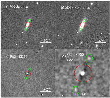
Figure 9. Example of difference imaging follow-up photometry for a nuclear transient using FPipe for SEDM on the P60 telescope. We use the TDE iPTF16fnl (Blagorodnova et al. 2017) as an example. Panel (a) shows the first P60 g-band follow-up image from the RC. The position of the transient is indicated by a red circle. Panel (b) shows the corresponding SDSS reference image. Panel (c) shows the resulting difference image between the RC exposure and the SDSS image after registration; PSF; and zeropoint matching. In Panel (d), we show the result of inserting two simulated sources with g-band magnitude of 22 mag in the image shown in (a) at the position of the green circles and redoing the subtraction procedure.
Download figure:
Standard image High-resolution image4.2. Integral Field Unit
The SEDM IFU data reduction pipeline (DRP) operates automatically to reduce the images taken by the IFU camera. The processing flow is shown in Figure 10. The processing consists of basic image reduction, then defining the IFU spatial and wavelength geometry followed by the spectral reduction and extraction stage. Extracted spectra are then calibrated using an inverse sensitivity curve that is generated from spectrophotometric standard star observations.
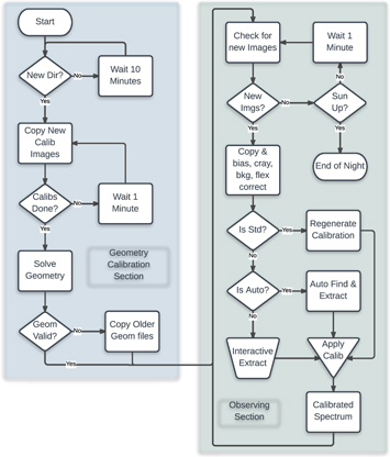
Figure 10. Data flow for the nightly IFU data reduction pipeline. The geometry calibration section is done late in the afternoon, while the observing section is done after sunset.
Download figure:
Standard image High-resolution imageAn alternative pipeline for SEDM was developed in the MATLAB environment and is available as part of the MATLAB Astronomy & Astrophysics Toolbox14 (Ofek 2014). This pipeline was used mainly for studying how to reduce the SEDM data given the challenges in wavelength calibration and background subtraction. The following describes the python pipeline.
4.2.1. Basic Reduction
The basic calibration set is taken during the late afternoon and consists of a set of bias frames; two sets of dome flats illuminated by a halogen lamp and by a Xe lamp; and two sets of internal arcs illuminated by Hg and Cd arc lamps. All these calibration images are taken with the telescope at the same position to minimize flexure offsets. Initially, the bias images are combined into a single master bias, which is then subtracted from all images. This is followed by a cosmic ray rejection stage that uses the lacosmicx15 python package. This package runs using cython, which makes this step faster than other cosmic ray rejection routines that run in native python. We tune the parameters such that the peaks of the spaxels are not rejected by using the gaussy PSF model that assumes that real objects have a Gaussian shape in the y-direction, but are extended in the x-direction. Once all the required calibration frames are reduced, the spatial and wavelength geometry can be defined.
4.2.2. Geometry Definition
The geometry definition stage uses a set of seven dome-flat images to define the spatial location of the spectral traces in the CCD pixel coordinate system. Arc-lamp image sets of Hg, Cd, and Xe arcs, shown in Figure 11 are used to define the wavelength solution for each individual trace. The geometry is established using the following steps:
- Spaxel location. The spectral traces, or spaxels, are determined using the dome flats. Five exposures of the dome-flat patch, illuminated by a halogen lamp, are taken and combined to remove cosmic rays and improve the S/N of the image. SExtractor is used to identify each spaxel segment in the image. These segments each have a unique segment ID and are used to derive the geometric properties of each spaxel. Each spaxel is fit with a second order polynomial to derive the spaxel ridge line as a function of CCD X and Y-pixel position. The width of the spaxel is retained as well. Since the blue illumination from the halogen lamp is low, the fits are extrapolated into the blue up to 350 nm. Using a very low-order polynomial ensures that this will not produce spurious results. The master dome-flat image with spaxel fits overlaid is shown in Figure 11(a).
- Rough wavelengths. Five Hg arc-lamp images are combined to form a master image. The brightest Hg lines are then identified in each spaxel trace, yielding a preliminary wavelength solution for each trace (see Figure 11(b)).
- Fine wavelengths. Five each of Xe and Cd arc images are combined to yield master calibration images that are analyzed to produce a refined wavelength solution for each trace (see Figures 11(c) and (d), and Figure 12). Spectra are extracted along each trace and each of the brightest individual lines are fit with a Gaussian to obtain the line center in pixels. Up to ten line positions from the Hg, Xe, and Cd arcs are fit to the known line wavelengths with a fourth-order Chebyshev polynomial. Figure 12 shows a typical trace with pixel positions on the Y-axis and wavelengths on the X-axis with the source of the individual lines indicated by color and shape and the resulting fit shown as the orange line.The median rms for the wavelength fit residuals of all spaxels is typically 0.3 nm. This corresponds to a redshift error of 5 × 10⁻⁴ at the approximate central wavelength of 600 nm. As our goal is the rapid typing of transients and selection for more detailed follow-up, which would include higher-resolution spectroscopy, hence, more accurate redshifts, this wavelength solution error is well within our error budget.
- Spatial projection. This fine wavelength solution is de-projected using the known geometry of the hexagonal microlenses to derive an X, Y position for each trace, relative to the spaxel closest to the center of the MLA, at a specific wavelength in the FOV of the IFU. These coordinates are recorded in pixels relative to the detector frame and in arcseconds relative to the center of the IFU.

Figure 11. Detail of the four calibration master images used to calibrate the IFU geometry, zoomed to show an individual spaxel and flipped in X so that wavelength increases toward the right. Panel (a) shows the dome-flat with trace fits over-plotted in blue, with a single trace highlighted in red. The initial and final wavelengths for the highlighted trace are annotated in white. Panel (b) shows the Hg arc image with the red highlighted trace indicating the alignment and extraction of the arc spectrum used to solve the preliminary wavelength solution. The four brightest Hg lines used for the first fit are shown with green, yellow, red, and magenta circles around them. Panel (c) shows the Xe arc spectrum used to define the long wavelength end of the geometry. Panel (d) shows the Cd arc spectrum used to refine the overall wavelength solution by providing more samples of lines at intermediate wavelengths.
Download figure:
Standard image High-resolution image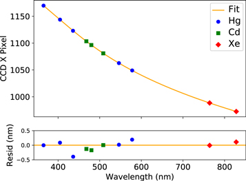
Figure 12. Example wavelength fit for a typical trace. A fourth-order Chebyshev polynomial was used to fit (orange line) the Hg lines (blue circles), the Cd lines (green squares), and the Xe lines (red diamonds). The wavelength residuals in nm are shown in the bottom panel.
Download figure:
Standard image High-resolution image4.2.3. Object Extraction
Once the geometric mapping of the spatial and spectral dimensions are defined, science observations can be reduced and spectrally extracted using the following steps:
- Flexure correction. As the telescope is moved around the sky, the flexure in the spectrograph can cause the spectrum to shift on the detector with small offsets. To derive this value, science images are first registered with the spatial and spectral geometry solution for the night. This is done in the Y-pixel direction by comparing spaxel locations in the master dome flat with those in the science images as delineated by the sky spectra to derive a master flexure offset in the Y-direction. This shift has a typical intranight variation of ≃0.5 pix. For the X-axis, or spectral direction, flexure is measured using one or both of two bright, relatively isolated sky lines at 557.7 nm (OI) and 589.6 nm (Na). This offset is typically less than 2 nm and the two lines (when both are measurable) typically agree to within the errors in the wavelength solution (0.3 nm). All subsequent extraction operations use these flexure correction values to extract the spectrum from a given science image.
- Background subtraction. An iterative background subtraction method is applied to remove scattered light from the IFU images. First, the flexure corrected spaxel locations are used to mask IFU image pixels that have been directly illuminated from the IFU. The unmasked region is assumed to contain only scattered light and is convolved with a 2D smoothing Gaussian kernel of 17 pixels width with successive surface fits for five iterations until a good map of scattered light is obtained. This is written out and subtracted from the science image.
- Sky Subtraction. For fainter objects (
 mag), a pair of images is obtained with a small (≈7'') pointing offset such that the object in one image falls on a background region in the other. The two images are then subtracted from one another to improve the target's contrast against the sky (see Section 3.2).
 - Spaxel extraction. All the spaxels for a given image are extracted by using the traces as defined by the master dome and corrected by the flexure values. A raw spectrum for each spaxel is built up by moving along the spaxel trace one pixel at a time in the X or spectral direction and performing a weighted sum of the image spaxels in the Y-direction extending above and below the trace center by three pixels (for a total of seven pixels). The weighting is calculated from a normalized Gaussian with same σ as the trace in the master dome-flat image. This weighting minimizes the contamination from neighboring spaxels. The flat-field value is also divided out at this time. The spaxels for the variance image are extracted with the identical method so the SNR can be calculated for each extracted spectrum.
- Object/Sky-host location. The light for the science object falls on a subset of all the spaxels, which need to be extracted along with the sky/host spaxels. Prior to object selection, a pseudo-image is formed by collapsing all the spaxels in wavelength from 650 to 700 nm, near the peak response of the IFU system. For bright ( mag) objects, an automatic object detection algorithm is then applied to the pseudo-image and fit with a 2D Gaussian to derive the extraction aperture. The sky spaxels are then defined based on the object extraction aperture. If the object is a bright, isolated stellar source, then all non-object spaxels are used to derive the sky spectrum, after applying a 3σ rejection criterion. For all other objects, the sky annulus is defined by extending the source aperture by 3'' and excluding the inner object spaxels. This is also applied to A and B image pairs despite of the former sky subtraction step, due to the need to also subtract the host-galaxy light.
- Interactive aperture placement. Because the offsets for the A/B pair images are adjusted for each individual object, and due to the small FOV of the IFU, which precludes a direct astrometric solution, these apertures are currently placed interactively. A graphical user interface (GUI) displays the pseudo-image with an aperture that tracks the mouse movement. Once the aperture is correctly placed, based on finder charts of the object, a mouse click registers the object location. The GUI also provides keystrokes to expand, or shrink the aperture, and to adjust the axial ratio and position angle of the aperture.Figure 13 shows the capabilities of the SEDM to extract both object and host spectra. All spaxels within the FOV are eligible for extraction. At the top left, a Type Ia SN, iPTF15drk, is shown in the SEDM pseudo-image with the A and B apertures indicated. The resulting spectrum is shown in the top right plot. The bottom left plot shows the apertures for the host galaxy and the bottom right shows the resulting spectrum. This capability is useful for checking the redshift derived from the SN and also for checking the host subtraction.
- Spectrum extraction. If the object is a standard star, then the Gaussian fit is extended to include 99.99% of the light and each spaxel is used to calculate the mean spectrum. If the object is not a standard, then the flux for each spaxel is summed between 500 and 900 nm and this total flux is used to rank order the spaxels. The brightest 70% of the spaxels are retained for determining the final spectrum. This prevents the faintest spaxels from adding noise to the final spectrum. The mean spectrum is then calculated for both the object and sky/host spaxels. The sky/host spectrum is then subtracted from the object spectrum and the object spectrum is scaled by the number of spaxels used. The error spectrum is calculated from the variance image spaxels corresponding to the object and sky spaxels used in the object image.


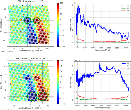
Figure 13. Extraction of SN and Host spectra for iPTF15drk, a Type Ia SN. SN is at the top and host galaxy is at the bottom. The color scale for the images on the left is arbitrary relative intensity, with red values positive (A exposure) and blue values being negative (B exposure). The right panels show the spectrum extracted for each aperture position.
Download figure:
Standard image High-resolution image4.3. Calibration
The flux calibration for SEDM is done using a set of spectrophotometric standard stars, shown in Table 3. The standards are observed and extracted as defined in the previous subsection. The reference flux for the standard is re-sampled onto the SEDM IFU wavelength scale, extinction corrected, and compared with the instrumental spectrum of the standard to derive an inverse sensitivity curve. This data then is used to convert any instrumental spectrum into a flux-calibrated spectrum. Generally, one standard is taken at the beginning of the night during late twilight. In addition, anywhere from one to five spectrophotometric stars are observed during the night. After each standard star is observed, the ensemble of observations is updated to form the mean calibration for the night.
Table 3. List of Spectroscopic Standard Stars Routinely Used for Flux Calibration by the IFU Pipeline
| Name | R.A. | Decl. | V (mag) | Type |
|---|---|---|---|---|
| BD+25d4655 | 21:59:42.02 | +26:25:58.1 | 9.76 | O |
| BD+28d4211 | 21:51:11.07 | +28:51:51.8 | 10.51 | Op |
| BD+33d2642 | 15:51:59.86 | +32:56:54.8 | 10.81 | B2IV |
| BD+75d325 | 08:10:49.31 | +74:57:57.5 | 9.54 | O5p |
| Feige110 | 23:19:58.39 | −05:09:55.8 | 11.82 | DOp |
| Feige34 | 10:39:36.71 | +43:06:10.1 | 11.18 | DO |
| GD50 | 03:48:50.06 | −00:58:30.4 | 14.06 | DA2 |
| HZ2 | 04:12:43.51 | +11:51:50.4 | 13.86 | DA3 |
| HZ4 | 03:55:21.70 | +09:47:18.7 | 14.51 | DA4 |
| LB227 | 04:09:28.76 | +17:07:54.4 | 15.32 | DA4 |
Download table as: ASCIITypeset image
5. Performance
5.1. Rainbow Camera
The performance of the RC has been computed using aperture magnitude on isolated (within 10 arcsec) stellar objects, contained in the SDSS and PS1 catalogs. For an exposure of 180 s, the average S/N for each filter and magnitude range is shown in Table 4. Figure 14 also shows the effect of the FWHM. The stars for this calculation were selected to have a magnitude in the range 13–20.5 in all four bands and were observed at airmass below 2.
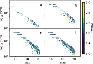
Figure 14. S/N for each filter for a 180 s exposure. The color indicates the FWHM on the exposure. Only observations with airmass <2 have been included into the plot.
Download figure:
Standard image High-resolution imageTable 4. Average S/N for Stars Within Each Magnitude Bin. We Include Only Isolated Point-like Sources. The Results are Computed for an Exposure Time of 180 s
| Filter | 17–18 | 18–19 | 19–20 | 20–20.5 |
|---|---|---|---|---|
| [mag] | [mag] | [mag] | [mag] | |
| u' | 55 | 30 | 20 | 12 |
| g' | 180 | 85 | 40 | 30 |
| r' | 135 | 70 | 30 | 23 |
| i' | 120 | 60 | 30 | 20 |
Download table as: ASCIITypeset image
5.2. Integral Field Unit
The IFU was designed to cover a wavelength range from 350 to 1100 nm. By comparing standard star observations with their calibrated fluxes, we find that the IFU total system response (telescope excluded) peaks at ∼9% between 550 and 725 nm (see Figure 15). The blue response falls rapidly below 400 nm. As a result, we typically do not use wavelengths below 400 nm for object classification.
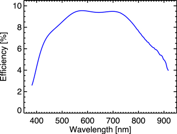
Figure 15. IFU efficiency in percent as a function of wavelength in Å derived from a 300 s exposure of the standard star Feige110. We assume an area of 18,000 cm2 for the P60 and an overall reflectivity of 82% and we correct for atmospheric extinction at Palomar (Hayes & Latham 1975).
Download figure:
Standard image High-resolution imageThe average S/N for the IFU is shown in Table 5. The S/N depends not only on the system throughput, but also on any component of scattered light we have in the system. Because of this scatter, we require to use the A/B method for sky subtraction, which currently reduces our sensitivity by a factor of  .
.
Table 5. Average S/N for Objects Within Each Magnitude Bin. The Results are Computed for an Exposure Time of 3600 s
| Wl. Range | 16–17 | 17–18 | 18–19 | 19–20 |
|---|---|---|---|---|
| [nm] | [mag] | [mag] | [mag] | [mag] |
| 400–500 | 11.3 | 10.2 | 7.2 | 3.4 |
| 500–800 | 20.3 | 18.0 | 10.1 | 5.5 |
| 800–900 | 18.6 | 15.9 | 5.8 | 3.1 |
Download table as: ASCIITypeset image
The microlens separation projected on the sky is 0.64'' in the RA direction and 0.56'' in the Dec direction. For the median seeing on P60 of 1.68'', we expect the PSF to be oversampled, which can also lead to an additional reduction in S/N. Figure 16 shows the curve of growth for a standard star normalized to the 500–600 nm bandpass. Half of the light for this bandpass is contained within an aperture with a semimajor axis of 0.65'', which is equivalent to a FWHM of 1.3''.
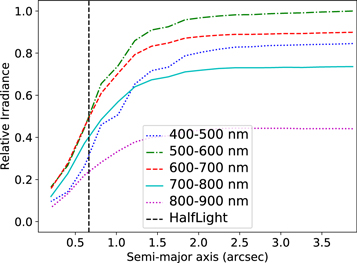
Figure 16. Curve of growth for IFU observation of Feige 110 for five wavelength bins. The half-light radius is indicated by the vertical dashed line and is equivalent to a seeing FWHM of 1.3''.
Download figure:
Standard image High-resolution imageWe calculate the S/N of the extracted SEDM spectra in the following manner. During reduction, we create a variance image which includes the Poisson noise from the signal and the read noise per pixel. This is calculated by simply adding the square of the read-out noise (5 × 5 = 25e−2 to the input bias-subtracted image. When the object and sky spaxels are identified prior to extraction, these same spaxels in the variance image are used to calculate the extracted variance spectrum. The object variance and the sky variance are added together so we account for both object and sky sources of uncertainty (unless we turn off the sky subtraction, in which case we just use the object variance). The noise in the spectrum is then simply the square root of the variance spectrum. This estimation does not include systematic errors, such as the ones cause by the scattered light.
As stated in Section 1, our design goal for the SEDM was to achieve a S/N of ∼5 for an object with an r-band magnitude of 20.5 in an exposure of 3600 s. Table 5 gives the average S/N for 43 extracted spectra for r-band magnitudes from 16 to 20 in each of three wavelength bins. This shows that we are consistently achieving the target S/N for objects with r magnitudes of 19.5; however, it is unlikely that we are achieving this goal for objects with r-band magnitudes fainter than 20.5. The 43 objects used for this calculation span a range of types, from bright, stellar, non-variable sources, to fainter, host-involved transients.
5.3. Improving SEDM IFU Optical Transmission
The optical modeling of the throughput for IFU predicted an efficiency >40% from 450 nm–750 nm. However, the measured efficiency on-sky appears to be about a factor of four less (see Figure 15). An investigation of this situation was conducted in the summer of 2017 at the Caltech Optical Observatory laboratories. The procedure involved the total disassembly of the optical system and the evaluation of the spectral transmission values for each component. The camera and optical collimator assemblies were tested as units, so as to not disturb their internal alignments.
This exercise determined that the integral-field hexagonal MLA contributed the majority of all optical losses. This array has a corner-to-corner diameter of 592 μm (0.74'') and focal length of 2660 μm, resulting in a fast-focal ratio of f/4.5. Closer examination of this array showed that there was an approximately 62 μm (radial) width dead-band on either side of the microlens boundaries. Optical light falling on this "gap" is not cleanly directed into desired micro-pupils, but rather is extensively scattered. The final measured median image size at the MLA is 2.2'' FWHM, implying that the dead-band scatters 20% of the total area of the image in an unpredictable manner. Such scatter removes signal from the micro-pupils, but also widely disperses unwanted photons into the spectrograph focal plane. A review of the original vendor procurement specification called out a maximum fill-factor of 95%, suggesting that the usable areal fraction of each microlens was fabricated on a best-effort basis, and only 80% effective fill factor was obtained.
In response to these investigations, we intend to seek a new alternative MLA vendor capable to delivering a smaller dead-band. While the original hexagonal MLA design choice was made in an attempt to ease the optical fabrication requirement for vendors, we believe greater experience within the community with high-fill-factor square microlens arrays now warrants investigation of such a design change. At the time of this writing, the vendor JENOPTIK16 has quoted a minimum 98% fill-factor square f/4.5 microlens for SEDM. Currently, we are seeking independent measurement verification of this performance to evaluate its suitability.
6. Examples and Early Science
SEDM began routine operations in late 2016 April as a shared facility on P60, along with the GRB imaging photometer. In 20196 August, it was designated as the primary instrument on the telescope. The SEDM has been in continuous use until the end of 2017 February, when the instrument was taken off for improvements. Over this total period of 10 months, the SEDM has obtained spectra of 1660 astrophysical sources, of which 465 corresponded to iPTF transient objects. The usage of the instrument has allowed us to increase the number of classifications by 25%–40% compared with previous years (2009–2015).
Currently, the spectroscopic targets for SEDM observations are specified on a nightly basis. However, a major strength of the SEDM is its low latency, defined as the time between a request for observations and spectral classification. Currently, we are implementing a target-of-opportunity mode in which SEDM observations can be scheduled immediately and observations undertaken within minutes (e.g., GRB afterglows or kilonovae).
The latency of the observations over the last two months is shown in Figure 17. For all transients with an SEDM spectrum, around one-third of them were observed within a day of their discovery, half of them in less than 2.5 days and a two thirds within the first five days of discovery. Some of the delays in obtaining a spectrum are due to inclement weather conditions, while others are related to human selection criteria or the shared usage of SEDM with other research groups. Overall, if we compare the latency for other transients observed with spectrographs on larger telescopes available to the PTF group (i.e., Palomar Hale telescope, Keck, DCT, Gemini, NOT, or APO), only 20% were classified within a day of their discovery, and the median delay time raises to four days.

Figure 17. Normalized histogram of the time elapsed between the date of discovery for a transient, and the date of the first spectrum. Orange bars show the distribution of time for transients with SEDM spectra and the black line for other telescope facilities. The data for the latter were obtained from the PTF transient database.
Download figure:
Standard image High-resolution imageAmong the classified transients, as expected, the most common types were SN type Ia, followed by SN type II, AGN, stellar sources and cataclysmic variables (CVs). Examples of these spectra are shown in Figure 18 and the spectral log is shown in Table 6. Whenever available, Figure 18 also displays a spectrum taken at similar epoch with another instrument for comparison. The sample includes four SN type Ia with different magnitude ranges, four SN type II, a SN Ic, and a broad-lined SN Ibc. It also contains two novae, two CVs, and other less-frequent transients, such as a super-luminous supernova (SLSN) and a TDE.
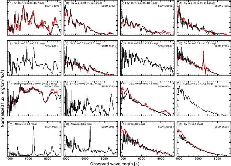
Figure 18. Sample of SEDM spectra for different transient types (black thick lines). Whenever available, long-slit spectroscopy taken at another telescope at a similar epoch is shown as a red thin line.
Download figure:
Standard image High-resolution imageTable 6. Spectroscopic Log for Figures 18, 19, and 20
| Panel | Classification | Redshift | Magnitude | tSEDM | Telescope | ttel |
|---|---|---|---|---|---|---|
| (mag) | (s) | +Instrument | (s) | |||
| Figure 18 | ||||||
| a | SN Ia | 0.02 | r = 16.7 | 1800 | FTN | 2700 |
| b | SN Ia | 0.04 | r = 17.3 | 2100 | P200 | 300 |
| c | SN Ia | 0.03 | r = 18.1 | 3600 | P200 | 300 |
| d | SN Ia | 0.12 | r = 19.6 | 2700 | P200 | 600 |
| e | SN II | 0.01 | r = 16.2 | 600 | ⋯ | ⋯ |
| f | SN II | 0.05 | r = 18.5 | 2100 | P200 | 300 |
| g | SN II | 0.07 | r = 19.4 | 3600 | ⋯ | ⋯ |
| h | SN IIn | 0.13 | r = 18.7 | 2700 | DCT | 900 |
| i | SN Ibc BL | 0.04 | r = 19.1 | 2700 | P200 | 600 |
| j | SN Ic | 0.02 | r = 18.7 | 2700 | ⋯ | ⋯ |
| k | TDE | 0.016 | r = 17.4 | 900 | P200 | 900 |
| l | SLSN | 0.1 | r = 17.3 | 1800 | ⋯ | ⋯ |
| m | Nova | 0 | r = 16.4 | 900 | ⋯ | ⋯ |
| n | Nova | 0 | r = 18.5 | 900 | ⋯ | ⋯ |
| o | CV | 0 | r = 18.5 | 3600 | P200 | 1500 |
| p | CV | 0 | r = 17.5 | 3600 | DCT | 1200 |
| Figure 19 | ||||||
| a | AGN | 0.082 | r = 17.0 | 3000 | Keck1 | 300 |
| b | AGN | 2.4 | r = 18.9 | 3000 | ⋯ | ⋯ |
| c | AGN | 0.04 | r = 14.75 | 3000 | DCT | 600 |
| d | AGN | 0.2 | r = 18.1 | 3000 | SDSS+2.5M | 6000 |
| e | Galaxy | 0.017 | r = 18.2 | 2700 | ⋯ | ⋯ |
| f | Galaxy | 0.048 | r = 17.4 | 2700 | P200 | 1200 |
| g | Galaxy | 0.027 | r = 12.5 | 2700 | SDSS+2.5M | 3600 |
| h | Galaxy | 0.02 | r = 18.0 | 2700 | P200 | 1200 |
| Figure 20 | ||||||
| a | O-type | 0 | r = 11.0 | 240 | ⋯ | ⋯ |
| b | A-type | 0 | r = 16.0 | 300 | ⋯ | ⋯ |
| c | F-type | 0 | r = 6.0 | 60 | ⋯ | ⋯ |
| d | G-type | 0 | r = 13.6 | 300 | ⋯ | ⋯ |
| e | K0-type | 0 | r = 11.5 | 300 | ⋯ | ⋯ |
| f | K5-type | 0 | r = 11.0 | 420 | ⋯ | ⋯ |
| g | M0-type | 0 | r = 18.2 | 2700 | ⋯ | ⋯ |
| h | M5-type | 0 | r = 17.5 | 300 | ⋯ | ⋯ |
Download table as: ASCIITypeset image
Up to date, the most notable discoveries of the SEDM are one of closest optical tidal disruption events: (iPTF16fnl; Blagorodnova et al. 2017); an unusual subclass of type Ia supernova 02cx-like (Miller et al. 2017); a rapidly turning-on quasar (iPTF16bco; Gezari et al. 2017); and a lensed SN type Ia (iPTF16geu; Goobar et al. 2017).
The SEDM can also be used for confirmation of redshifts of nearby (≲200 Mpc) star-forming galaxies. The typical precision (1σ) for the recession velocity inferred from the SEDM spectra is  and the accuracy is ∼250 km s−1. Figure 19 shows four examples of AGNs and four spectra of galaxies at different magnitudes. The spectra are adequate enough to allow us to distinguish between passive and active galaxies.
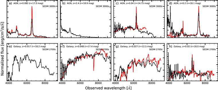
Figure 19. Sample of SEDM spectra (black line) for different AGNs and galaxies. Whenever available, long-slit spectroscopy taken at a similar epoch is shown as a red thin line.
Download figure:
Standard image High-resolution imageThe SEDM has been used to study stars both spectroscopically and photometrically. An example of spectroscopic observations of stellar sources is shown in the collage in Figure 20. The surprising success of the SEDM in determining effective temperature (via model fits to the data) have motivated us to embark on a project to quantitatively determine the precision of the SEDM in measuring the effective temperature as well as the degree of reliability of spectral classification. Additionally, the SEDM has also enabled a search for emission lines sources. Two new Be stars in the open cluster NGC 6830 were identified via their emission lines in Hα and absorption lines of Hβ, Hγ, He I λ4471 and Mg II λ4481 (Yu et al. 2016).
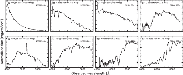
Figure 20. Sample of SEDM spectra for different stellar objects (black thick lines). Generally, the stellar sources have magnitudes between 11 and 18 mag. Panel e) shows an example of an emission-line star in the open cluster NGC 743.
Download figure:
Standard image High-resolution imageExamples of photometric stellar studies include detailed characterization of eclipses in close binary systems, such as the one shown in Figure 21, multi-band follow-up of binaries showing reflection effects from a hot compact companion and complementary observations for determination of periods for variable stars.

Figure 21. Light curve of an eclipsing binary system. The data shown was obtained with the SEDM aperture photometry pipeline. The exposure time was fixed to 60 s. The error bars are smaller than the size of the markers.
Download figure:
Standard image High-resolution image
7. Discussion and Conclusions
We have presented an overview of the instrumental design and operations of SEDM, a dedicated low-resolution IFU spectrograph on the Palomar 60-inch telescope. The instrument has been used for spectroscopic classification and photometric follow-up of iPTF transients discovered during 2016 and early 2017. Overall, the SEDM produces consistently classifiable spectra for targets brighter than R = 19.5 mag with exposure times of 3600 s or less. Although iPTF has a limiting magnitude about 1 mag deeper than that, discoveries made during PTF/iPTF era show that around one-third of all transients were detected with magnitudes <19.5 in either g- or R-band. Around 40% of all transients were brighter than 19.5 mag at peak, and therefore suitable for classification with SEDM. With an average rate of 10 spectra per night, the SEDM has proved to be a useful tool for the fast initial classification of candidates and photometric follow-up.
The versatility of the instrument allows it to be useful in numerous applications across different astronomical fields, beyond its initial application to transient astronomy. Given the larger sky coverage of ZTF over iPTF: 3760 deg2/h versus 247 deg2/h, we expect the SEDM will be continuously over-subscribed once the survey becomes operational.
Currently, there are around 40 optical operating telescopes larger than 3 m in the world. However, the number of smaller telescopes with diameters between 1–3 m, is much larger, around 150. Hence, the possibility to replicate the instrument on other 1–3 m class telescopes could alleviate the "follow-up drought," allowing new surveys to obtain a more complete characterization of discovered transients for a magnitude limited survey, providing unbiased statistical samples of numerous transient families in our nearby universe.
Footnotes
- 10
Source: http://www.rochesterastronomy.org.
- 11
- 12
- 13
The pipeline can also utilize PS1 image stacks as references. However, the PS1 filters are not as well matched to the filters mounted on the SEDM RC, resulting in considerably stronger residuals for bright point sources compared with when SDSS references are used.
- 14
- 15
- 16