
Abstract
Spatial relocalization of proteins is crucial for the correct functioning of living cells. An interesting example of spatial ordering is the light-induced clustering of plant photoreceptor proteins. Upon irradiation by white or red light, the red light-active phytochrome, phytochrome B, enters the nucleus and accumulates in large nuclear bodies (NBs). The underlying physical process of nuclear body formation remains unclear, but phytochrome B is thought to coagulate via a simple protein–protein binding process. We measure, for the first time, the distribution of the number of phytochrome B-containing NBs as well as their volume distribution. We show that the experimental data cannot be explained by a stochastic model of nuclear body formation via simple protein–protein binding processes using physically meaningful parameter values. Rather modelling suggests that the data is consistent with a two step process: a fast nucleation step leading to macroparticles followed by a subsequent slow step in which the macroparticles bind to form the nuclear body. An alternative explanation for the observed nuclear body distribution is that the phytochromes bind to a so far unknown molecular structure. We believe it is likely this result holds more generally for other nuclear body-forming plant photoreceptors and proteins.
Export citation and abstract BibTeX RIS

Original content from this work may be used under the terms of the Creative Commons Attribution 3.0 licence. Any further distribution of this work must maintain attribution to the author(s) and the title of the work, journal citation and DOI.
1. Introduction
Spatial distribution and movement of proteins play essential functional roles in signalling pathways of biological systems. On a cellular level such dynamic and stimulus-dependent localization patterns involve and comprise distinct but connected compartments like the cytosol and nucleus. In some prominent cases, sub-compartmental pools of proteins, both within the cytosol and nucleus, can be distinguished and addressed visually by microscopic techniques (for example, see figures 1(A) and (B) or the examples within [1, 2]). The formation of so-called nuclear bodies (NBs), in particular, is thought to be crucial for transcriptional regulation and chromatin dynamics, as has been observed in both mammalian and plant cells [1, 3]. However, how such large structures within the nuclei of cells (in some cases observed to be between 1 and 2 μm [4]) form spontaneously is currently an open question, particularly in plants.

Figure 1. Exemplary nucleus with late nuclear bodies of an Arabidopsis thaliana seedling after 24 h of red light treatment. (A) Epifluorescence analysis of phyB-YFP fusion proteins, (B) bright-field image of the nuclear area depicted in A. Scale bar represents 10 μm. (C) Schematic of the phytochrome nuclear body forming process. Upon light irradiation (red arrow: 667 nm, dark-red arrow: 730 nm wavelength of the incident light) the phytochromes are transformed from the Pr to the Pfr state and transported into the nucleus where they aggregate into nuclear bodies.
Download figure:
Standard image High-resolution imageA classic observation of NBs comes from investigations into the functions of photoreceptors in the model plant Arabidopsis thaliana. Across evolution, several classes of photosensory proteins arose covering a wavelength range from around 280 nm to 760 nm. Among these families, the most prominent photoreceptors are UVR-8 that senses UV-B radiation [5], the blue light-detecting cryptochromes (crys) [6, 7] and phototropins [8], and phytochromes (phys) that mainly act under red and far-red irradiation [9]. Photoreceptors change conformation upon being activated by specific wavelengths of light and are subsequently transported to the nucleus where they form NBs, also sometimes referred to as spots or speckles. Notably, cryptochrome 2 (cry2) and two members of the phytochrome family, the light-labile phytochrome A (phyA) and light-stable phytochrome B (phyB), have been shown to form NBs when exposed to the required activating light conditions [10–16].
Here we shall specifically focus on the formation of NBs by phyB and hence we now give some further relevant details of the processes involved. phyB photoreceptors are present in vivo as dimers. Upon irradiation by red light of wavelength 667 nm, they switch from their inactive conformational state (denoted as Pr) to their active conformational state (denoted as Pfr). The reverse transition occurs in darkness via thermal relaxation and also if the phyB dimers are exposed to far-red light of wavelength 730 nm (for a review, see [9]). Hence the steady-state ratio of active molecules within the molecular population is dependent on the spectral composition of the incident light [17, 18]. The active form of phyB is subsequently transported to the nucleus where it leads to the formation of NBs (see figure 1(C) for an illustration).
There are at least two different types of light-mediated NBs which have been described, often referred to as early and late NBs. Early NBs are transient and small complexes which emerge within seconds after Pfr formation. These structures depend on and contain the bHLH transcription factor PHYTOCHROME INTERACTING FACTOR 3 (PIF3). These early NBs are essential to control the abundance of the signalling component PIF3 due to physical interaction with phyB Pfr that results in phosporylation and proteasomal degradation of the transcription factor [19, 20]. The second type of nuclear body called late NBs are stable and start to form after an hour of continuous irradiation (figure 1) [10, 13, 21]. The molecular function of the late and bigger phyB NBs in signalling is far from being well understood although a number of hypotheses have been put forward [22, 23]. Crucially, though, the formation of phyB-containing nuclear structures has been shown to be important for regulation of stem elongation [24, 25].
In this study, we investigate the formation of the late phyB NBs. In particular, we aim to answer the question whether the large phyB NBs can be formed by simple protein binding, i.e. how likely is it that the large NBs are mere phytochrome aggregations resulting from binding one phyB after the other? We combine experimentally-obtained data detailing the size and number of these bodies with data from the literature and mathematical modelling. Based on our theoretical analysis, we discuss the requirements for the assembly and formation of phyB NBs. Although we focus on the case of phyB within Arabidopsis thaliana cells, we believe our results are generalisable to other photoreceptor systems that form NBs. Crucially, our analysis suggests that NB formation does not happen through simple diffusive protein–protein interactions, leading us to conclude that other processes lie behind the appearance of NBs.
2. Experimental measurements
In order to gain insight into the NB formation process, we measured the distributions of NB size and number per cell. To this end, we used 4 d old phyB:GFP/ phyAphyB Arabidopsis thaliana seedlings. After germination, seedlings were transferred to glass slides and optical sections were collected under continuous red light irradiation by confocal microscopy. Images were exported and analyzed with ImageJ 1.41o software by creating Z-Projection of the 3D data stacks and determining the particle cross-sectional area after image processing. For more information about growth conditions and image acquisition see the appendix. The obtained images are consistent with NBs of approximately spherical shape. From the measured cross-sections we hence obtained the corresponding volume of each NB. Further, we counted the number of phyB NBs in each cell. In total we measured 1074 NBs from 175 nuclei.
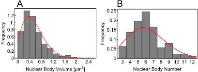
The resulting size and number distributions are shown in figure 2. From these distributions one can calculate some basic averaged quantities: the mean number of NBs in a nucleus is approximatively 6 and the mean volume of an NB is 0.55 μm3, corresponding to a sphere with diameter approximately 1 μm. Thus, given that the diameter of a molecule is on the order of nanometers, it is clear that a micron sized NB must consist of a huge number of molecules (approximately 106–109). These averages however are not the whole story. In particular it is plausible that the shapes of the distributions in figure 2 reflect key information regarding the nature of the underlying processes leading to NB formation. This question is investigated next by means of mathematical modelling.
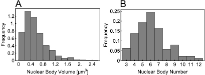
Figure 2. In (A) the histogram shows the experimentally measured volume distribution. In (B) the histogram shows the distribution of the number of phyB NBs found in the individual nuclei.
Download figure:
Standard image High-resolution image3. A mathematical model of NB formation
In this section we hypothesize the formation process of NBs and use statistical physics to derive expressions describing the measured distributions. By comparison of the key features of these distributions with the experimentally derived ones, we deduce which processes are compatible with NB formation and which are not.
We first make some simplifying assumptions. Since gene expression involves a large number of steps, it is typically considered to be much slower than direct protein–protein interactions [26] and hence a reasonable assumption is that light-activated dimers are immediately available in both the cytoplasm and nucleus. Next we assume that NBs are formed solely of active phyB dimer molecules and each NB can grow and shrink by binding and unbinding single active phyB molecules (those in the Pfr state induced by light-activation). Hence we shall refer to an active phyB molecule as the fundamental building block. The reaction scheme underlying the aforementioned processes is given by:
where S1 is the fundamental building block and Sm is a complex composed of m building blocks. All species described reside in the nucleus. The first reversible reaction describes the transport of the building block from the cytoplasm to the nucleus with rate kin and from the nucleus to the cytoplasm with rate kout; transport occurs via diffusion and active transport mechanisms. The rest of the reactions describe the growing and shrinking of complexes by one building block at a time, where a complex Si is equated with a NB composed of i building blocks.
The reaction rates  generally depend on the size of the NBs. Specifically we assume a power law form for the rates:
If we assume that the NB and the building blocks are rigid spherical particles and that they diffuse in the nucleus then, from Smoluchowski's theory of reaction rates, the association rates are volume independent for reaction-limited kinetics (implying  ) and proportional to the radius of the NB (implying
  since m is proportional to the volume of the NB) for diffusion-limited kinetics [27]. Dissociation could occur by a building block dissociating from anywhere in the volume of the NB (implying
  ) or perhaps only from the surface of the NB (implying
  ). Generally α and β depend on the shape and rigidity of the NB, number and location of preferential binding sites as well as on the physics governing the association and dissociation processes. Such detailed information about NBs is presently unavailable and hence we shall leave α and β general. The parameters a and b are the association and dissociation rates having the standard units
 ![$[a]={\rm (Ms)}^{-1}$](https://content.cld.iop.org/journals/1478-3975/15/5/056003/revision2/pbaac193ieqn006.gif) and
and ![$[b]={\rm s}^{-1}$](https://content.cld.iop.org/journals/1478-3975/15/5/056003/revision2/pbaac193ieqn007.gif) (M: molar, s: seconds), respectively.
(M: molar, s: seconds), respectively.
Since the late phyB NBs which we are modelling, are stable under constant experimental conditions [13, 25], we will be deriving expressions for the number and size distributions of the NBs in steady-state conditions.
We start by stating a general result. Consider a general chemical reaction system involving N species and composed of reversible reactions such that:

where j is a reaction index varying from 1 to the total number of reactions R, Xi denotes the ith chemical species and sij and rij are the integer stoichiometric coefficients. Say this chemical reaction system occurs in some reaction volume Ω and that there are A chemical conservation laws of the form:
where ni is the number of molecules of species Xi, and the c's and M's are some time-independent constants.
The chemical master equation provides a rigorous description of the well-mixed stochastic dynamics of the reaction system. Specifically it describes the time-evolution of the probability distribution of states of the system [28]. Van Kampen showed [29] that the steady-state solution of the chemical master equation for the general chemical system above is given by a Poisson distribution constrained by the existing chemical conservation laws:
This equilibrium solution exists provided the following condition from the law of mass action is fulfilled for each reversible pair of reactions:
This result can also be extended to the spatial case [30] but here we shall use the non-spatial version for simplicity, i.e. assuming well-mixed conditions inside the nucleus.
Now we can apply the general result above to the reaction scheme (1) that we previously proposed as a simple model of NB formation. This reaction scheme is purely composed of reversible reactions and hence is a specific case of the general reaction scheme (3). It can be easily verified from the rate equations that because of the reaction modelling the input and output of S1 (to and from the nucleus) our reaction scheme (1) has no associated chemical conservation laws. Thus it follows by equation (5) that the steady-state solution of the chemical master equation describing our simple model of NB formation is a Poisson distribution given by:
where  is the probability of observing the state
  , i.e. is the probability of observing n1 NBs composed of one building block, n2 NBs composed of two building blocks, etc. Note that the index j in the above equation can take values to infinity because there is, in principle, no limit to the size of an NB attained through the one-by-one binding process described by scheme (1). It then follows that equation (6) for the NB formation process is given by:

where we used equation (2). Solving this set of equations gives us:
where  . Substituting equation (9) in equation (7) we obtain the equilibrium NB distribution:

where we have defined the dimensionless constants  and
and  . We next use equa-tion (10) to derive expressions for our experimental observables: the size and number distributions of NBs.
3.1. The size distribution
Experimentally we constructed the histogram in figure 2(A) by calculating the number of NBs of a specific size (using data from all nuclei) divided by the total number of NB measured from all nuclei. This corresponds to the size distribution for the NBs given by:
 is the expectation value of the number of nuclear bodies of size m. The experimental estimator for this distribution reads:
where Z = 175 (the number of nuclei used in the experimental analysis) and  is the number of NBs of size m in nucleus i. Using equation (10) we find for the frequency distribution of the NB size:
where  is the expectation of the total number of NBs in a nucleus. Since we observed that NBs are rather large and consist of millions of proteins, we approximate the factorial in equation (13) using the Stirling approximation leading to:
Finally we change from the distribution over m to a distribution over the volume of the NB  since the latter is experimentally observable. We assume that the NBs are spheres composed of randomly packed spherical fundamental building blocks of volume
  . Then it follows that
  where ν accounts for the random spatial packing of spheres, i.e.
  [31]. Since we are taking our fundamental building block to be a phyB dimeric molecule (∼240 kDa),
  is estimated to be 2.7 × 10⁻⁷ μm3. Hence the volume distribution is given by:
where  and
and  .
.
3.2. The number distribution
The number distribution  accounts for the probability to observe a given number Ns NBs:
where  denotes the Kronecker function (
 for i = j and
  otherwise). The easiest manner to include the constraint is to use the generating function method, as follows.
One defines the generating function as  which simplifies to:
Here we used the fact that  (see equation (7)) can be written as a product of exponentials
  where
where  . Transforming back to the number distribution one finally obtains:
which is a Poissonian distribution with mean  .
.
4. Estimating association and dissociation parameters from experimental measurements
We fit the experimental data using the distributions given by equations (15) and (18). The unknown parameters were estimated using maximum likelihood methods [32], as follows. Fitting equation (18) to the experimentally measured number distribution we obtained an estimate for  . Fitting equation (15) to the experimentally measured volume distribution we obtained estimates for δ, Δ, γ and the product
  using
using  and
and  10−7 μm3. Using the estimate for
  we then obtained an estimate for K. For the maximum likelihood we used the fitdistr of the MASS package implemented in R [33]. For estimation of the error bounds we used standard uncertainty propagation [34]. The average number of fundamental building blocks (phyB dimers) per NB denoted as
  can then be computed from equation (13). The resulting estimated parameter values are given in table 1.
Table 1. Estimated parameters from experimental data using maximum likelihood and the analytical size and number distribution given by equations (15) and (18). The estimation for a and b is based on the estimation of K and a previous measurement of the dissociation rate using FRAP [24] (see text).
 |
 |
|---|---|
 |
 |
 |
 |
 |
 M M |
 |
 |
| a |  |
| b |  |
The association and dissociation rates a and b, respectively, cannot be estimated directly from the distributions. However, from previous experiments we estimated that the average dissociation rate from NBs is  min−1 [24]. This approximation is likely to be an upper limit, depending on the form of phyB Pfr-containing dimers [23]. From this we can estimate b:
 . Consequently, one obtains
  from the relation
  . Using an estimate for the reaction volume, i.e. the volume of the nucleus of Arabidopsis thaliana (
 m3 [35]), we obtain an estimate for the unscaled association rate in standard units:
  .
.
Given the estimated parameter values, the corresponding distributions are shown as red solid lines in figure 3.
Figure 3. Comparing the experimentally measured histograms for the volume (A) and the number (B) distribution with the corresponding analytical distributions (red solid lines) given by equations (15) and (18), respectively. The estimated best fit parameters used for the analytical distributions are given in table 1.
Download figure:
Standard image High-resolution image
5. Discussion
In this study we have, for the first time, presented distributions for the size and number of phyB-containing NBs within plant nuclei under red light (see figure 2). By fitting the experimentally measured frequency distributions (figure 3) using equations derived from our simplified mathematical model of phyB nuclear translocation and NB formation (equations (15) and (18)), we have estimated several parameters associated with NB formation (table 1).
These estimates enable us to make the important conclusion that the experimental data is not consistent with NBs being formed of fundamental building blocks composed of a phyB dimer and that the process leading to NB formation cannot be simply binding-unbinding. The detailed reasoning follows. The fundamental building block cannot be a phyB dimer because then our theory estimates about a million of them on average in each NB ( ) whereas it is known that on average plant cells have at most a few tens of thousands of phyB dimers [36]. The process cannot be simple binding-unbinding because the estimated association rate
  needed to build the NBs is two orders of magnitudes larger than the fastest known protein association rates, which is of the order of
  [37, 38].
A way around these two difficulties is as follows. Let us assume that the fundamental building units are considerably larger than a phytochrome dimer, that the interactions are still of the simple binding-unbinding type and that each NB is a random close-packed structure of the fundamental building blocks. If the fundamental building blocks are particles with approximate radius  , one finds for the association rate
  which is in the range of observed binding constants [37, 38]. This suggests that NB formation consists of two steps: an (so far) unobserved fast nucleation step leading to the formation of macroparticles with approximate radius
  , and a slow step in which the large NBs form due to binding of these macroparticles (similar to an Ostwald ripening mechanism [39]). There are at least two possibilities for how the macroparticles are formed in the first nucleation step: (i) phyB dimers aggregate into these macroparticles, and (ii) phyB dimers associate with other proteins to form the macroparticles. This is consistent with the fact that a number of different proteins have been found to co-localize within phyB-containing NBs, including PHYTOCHROME INTERACTING FACTORs, HEMERA, and cry2 [12, 19, 20, 40]. The two step NB formation process can be obtained by particular parameter choices and a generalisation of our reaction scheme (1) where we now allow reactions between complexes of size i and j to form a complex of size i + j.
Another possibility is that the NBs internal structure is not well approximated by random close-packing (as we have assumed thus far). For example they could be mostly hollow and/or the phytochromes bind to a so far unknown molecular structure. This would result in a substantially reduced number of phytochrome molecules per NB. This model of plant NB structure, whereby proteins are observed on the surface of the NBs, fits well with current ideas from other fields [2]. In these studies, the components that are internalised within NBs are referred to as 'seed' molecules, e.g. RNA and chromatin, and are thought to aid regulation of stress responses and coordinate cellular dynamics in changing environments [1–3, 41].
In conclusion, our findings indicate that the late phyB NBs cannot be formed by a simple binding process between phyB molecules. More detailed, microscopic studies will be required to elucidate the exact structure of phyB NBs and their constituent components in planta. Future research should aim to obtain a better understanding of the dynamics of NB formation and of the components co-existing within phyB NBs. This may help to elucidate whether these bodies function as transcriptional regulators, are important for protein sequestration/degradation, or a combination of the two to regulate plant development under changing environmental conditions.
Acknowledgments
RG acknowledges support by SULSA (Scottish Universities Life Science Alliance) and by FRIAS (Freiburg Institute for Advanced Studies). CF acknowledges support by the BMBF–Freiburg Initiative in Systems Biology grant 031392 and by HFSP Research grant RGP0025/2013. RWS is supported by FP7 Marie Curie Initial Training Network grant agreement number 316723 and EU Horizon 2020 grant agreement number 634942.
Appendix A. Plant material
Arabidopsis thaliana [ecotype Columbia] transgenic lines expressing the 35S:PHYB- GFP transgenes in phyA-211 phyB-9 background (B-GFP/A- B-) were sown on Petri dishes (9 cm diameter) containing 4 layers of filter paper (Macherey-Nagel, Germany) and 4.5 ml distilled water. After stratification (two days at 6 °C in darkness) uniform germination was induced by a 4 h white light treatment at 22 °C. Afterwards seedlings were grown at 22 °C in darkness for four days.
Appendix B. Image acquisition
For determination of nuclear body formation and size distribution, a confocal laser-scanning microscope LSM Meta 510 (Carl Zeiss) was used. Laser intensity and exposure time were adjusted to minimise photo-bleaching as well as for adequate dynamic range of GFP detection in order to avoid clipping. GFP was excited with an Ar-laser at 488 nm and detected at 510 nm–550 nm. After setting up the imaging system for optimal signal detection, all the relevant parameters, including laser output, binning, intensity, pinhole size and amplifier gain, were kept constant for imaging. Each experiment was performed at least twice independently. Seedlings were pre-irradiated with saturating red light (660 nm LED chamber, 26 μ mol m−2 s−1) for 24 h. Subsequently, seedlings were transferred to glass slides. For spatial resolution, around 7 optical sections were collected with 0.75 μm between consecutive sections. Multi-color images were acquired for detection of interfering signals by plastids and nuclear location. Confocal microscopy images (45.00 × 45.00 μm2;  pixels, 8-bit) were exported and analysed with ImageJ 1.41o software.
Appendix C. Image analysis and processing
Multi-color aquisitions were split into single channels before proceeding. A maximum projection image of the 3D data stacks was performed. An adequate threshold level was determined in a known range of pixel intensities by intensity histogram analysis and a binary image was created to highlight the nuclear body structures and to achieve a high signal-to-noise and signal-to-background ratio. The same range of pixel intensity was used for every set of image. After getting a binary picture with clearly distinguishable structures, the particle cross-sectional area (size: μm2, 0.1-infinity, 'Circularity' 0.01–1.00) was determined.