

Abstract
This report presents a simple model that describes the motion of a single Dictyostelium discoideum cell exposed to a traveling wave of cyclic adenosine monophosphate (cAMP). The model incorporates two types of responses to stimulation by cAMP: the changes in the polarity and motility of the cell. The periodic change in motility is assumed to be induced by periodic cAMP stimulation on the basis of previous experimental studies. Consequently, the net migration of the cell occurs in a particular direction with respect to wave propagation, which explains the migration of D. discoideum cells in aggregation. The wave period and the difference between the two response times are important parameters that determine the direction of migration. The theoretical prediction compared with experiments presented in another study. The transition from the single-cell state of the population of D. discoideum cells to the aggregation state is understood to be a specific example of spontaneous breakage of symmetry in biology.
Export citation and abstract BibTeX RIS
1. Introduction
Several types of cells can sense the presence of extracellular signal molecules and migrate in the direction of the concentration gradient of the signals. This phenomenon is known as chemotaxis and plays an important role in a variety of biological systems including mammalian neutrophils [1], fibroblasts [2], microglia [3], and cancerous cells [4]. Dictyostelium discoideum serves as an ideal model for the study of chemotaxis [5], and cyclic adenosine monophosphate (cAMP) is a chemoattractant for D. discoideum cells.
Starved D. discoideum cells aggregate and form multicellular slugs. The aggregation processes of D. discoideum cells are mediated by propagating waves of different concentrations of cAMP secreted by cells [5]. At the initiation of aggregation, the wave periods are approximately 10 min [6]. As time elapses, the wave periods progressively shorten to approximately 5 min [6–11]. The cells migrate toward the wave source [6–9] and then converge at the wave source [12].
The waveform of the cAMP wave is symmetrical and mono-phasic [9]. When the wave passes through the cell, the cell periodically experiences positive and negative gradients of cAMP concentration (figure 1(a)). If a cell only assesses the spatial gradient of cAMP waves and moves in the direction of higher concentrations, the movements toward and away from the wave source would cancel each other, thus resulting in a lack of net migration in any particular direction. However, cells actually move toward the wave source in an aggregation process. This inconsistency is known as the 'wave paradox [13].'

Figure 1. Schematic illustrations of the model. (a) A single chemotactic cell is exposed to a traveling wave of cAMP with the wavelength λ and the wave period T. The wave propagates from the right to the left with the speed  . The cell senses the gradient of the cAMP concentration and the temporal change in the cAMP concentration, and migrates to the left or right on the basis of these signals. (b) cAMP stimuli induce two different responses: changes in polarity and motility. Stimulation at a certain time, 0, induces a change in polarity at time
  and in motility at time
  [16]. In other words, the polarity and motility at time t are induced by stimulation at time
  and at time
  , respectively.
Download figure:
Standard image High-resolution imageWhile some models have been proposed on the basis of the adaptation mechanism of the cell [14–23], we now propose another mechanism that may solve the paradox. In particular, we present a highly simplified phenomenological model describing the chemotactic motion that incorporates response times to the periodic chemical signal. Our analysis reveals that the period of the cAMP waves and the difference in response times govern the direction and speed of cell migration. The theoretical results are compared with experimental data measured by Skoge et al [24]. The present model predicts the net migration away from the wave source for large wave periods while the adaptation mechanism predicts that cells move in the front of the wave and remain more or less stationary in the back of the wave, which always results in the net migration toward the wave source [15, 17].
2. Results
2.1. Model
We consider the motion of a single D. discoideum cell in one dimension exposed to a periodic traveling wave of cAMP concentration (figure 1(a)). The model equation in this study is such that the position of a single cell, x(t), is governed by the following equation of motion,
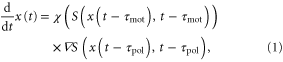
where  is a periodic function with respect to both x and t. This quantity indicates the strength of the stimulation, which is positively correlated with the concentration of cAMP. Therefore, S is assumed to be an increasing function of the concentration of cAMP. The function, χ, referred to as the chemotactic coefficient in what follows, is also a periodic function that increases when
 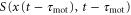 increases. The functional forms of S and χ are determined later. The biological meanings of the two parameters,
  and
and  , are explained in following paragraphs.
This model equation is constructed as follows (further mathematical derivation based on some experiments [16, 25–27] is shown in appendix
The polarity is a directional pseudopod extension toward the gradient of the cAMP concentration. This phenomenon is induced by the localization of proteins including phosphatidylinositol 3, 4, 5-trisphosphate along the plasma membrane resulting from sensing of the gradient of the cAMP concentration [32]. In the present model, we attribute the magnitude of this response to  . The parameter,
  , is introduced to incorporate the response time from stimulation to the change in the polarity.
The motility is the magnitude and the frequency of the pseudopod extension. Mathematically, the chemotactic coefficient, χ, describes the motility. We assume that the motility depends on the magnitude of the stimulation, S. Based on this assumption, the chemotactic coefficient, χ, oscillates with the same period as the periodic stimulation by cAMP, S. The parameter,  , is introduced to incorporate the response time from stimulation to the change in the motility.
The assumption of oscillatory behavior for the motility is supported by some previous studies. Soll et al measured the time series of the instantaneous velocity of a single D. discoideum cell in detail when the cell was exposed to temporally periodic changes in cAMP concentration in the absence of a spatial gradient [16, 25–27]. The magnitude of the instantaneous velocity oscillated with the same period as the extracellular cAMP concentration. This result implies that periodic stimulation by cAMP induces periodic changes in motility. In the situation we consider here, the cell is periodically stimulated by the traveling wave. Therefore, we assume that the chemotactic coefficient oscillates with the same period as the periodic stimulation. Because a significant constant phase difference between the oscillation of the extracellular cAMP concentration and that of the instantaneous velocity was observed in those experiments, the response time,  corresponding to the phase difference is introduced in the model.
2.2. Net migration
First, we consider a case in which the waveform of the stimulation is a sinusoid, namely

where λ and T denote the wavelength and the period, respectively. Save represents the average of the stimulation, and Sosc represents the amplitude of the oscillation, satisfying  . We determine the waveform (2) from previous experimental results [9, 16, 34, 35]. The concentration of the cAMP wave changes exponentially between 10−8 and 10−6 M, and the waveform is sharply peaked, which is well approximated by
 ![${\rm exp} [{\rm sin} \left( 2\pi x/\lambda +2\pi t/T \right)]$](https://content.cld.iop.org/journals/1478-3975/12/2/026004/revision1/pb510555ieqn15.gif) [9]. Additionally, the velocity of the cell varies roughly with the spatial gradient of the logarithm of the concentration [35]. Thus, we use a sinusoid for S. Note that, as we discuss later, the choice of the waveform is not essential to the result.
[9]. Additionally, the velocity of the cell varies roughly with the spatial gradient of the logarithm of the concentration [35]. Thus, we use a sinusoid for S. Note that, as we discuss later, the choice of the waveform is not essential to the result.
The chemotactic coefficient is also assumed to be a sinusoid, namely

where  and
and  are constant parameters satisfying the condition,
  . This assumption is derived from the observation that the amplitude of the fluctuations of the velocity of the cell is proportional to the logarithm of the wave amplitude of the cAMP concentration when there is no spatial gradient [16, 34].
We show that the propagation of the traveling wave induces a migration in one direction. We can generate the approximations  and
and  because the velocity of the traveling wave,
  μm min−1 [9], is much greater than the speed of the cell, which varies between 0 and 7 μm min−1 [16]. By substituting the equations (2) and (3) into the equation of motion (1), the velocity of a single cell is reduced to (further detailed derivation of equation (4) is shown in appendix
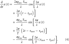
The third term on the right hand side of the equation (4) is a constant, whereas the first and second terms are periodic with respect to time as long as x(t) is treated as a constant during one wave period. Therefore, on the average over one wave period, the third term contributes to the translocation of the cell much more than the first and second terms. By eliminating those periodic terms, the averaged velocity,  , is obtained as follows

Figure 2 illustrates the numerical solution of the differential equation (1) for parameters typical in the aggregation state of a cell (see table 1). It is also apparent that the averaged velocity,  , well approximates the net migration of a cell.

Figure 2. Motion of D. discoideum cell in the aggregation state. We show the instantaneous velocity, v(t), and the position of a cell, x(t), with periodic stimulation by the cAMP wave. The average position,  , is calculated from the averaged velocity,
  , in equation (5). The red curve at the bottom represents stimulation by cAMP at the position, x(t). This curve is shown as a reference to compare the phases among oscillations of velocity, displacement, and stimulation.
Download figure:
Standard image High-resolution imageTable 1.
Typical values for D. discoideum cells in the aggregation process. They are used in a numerical calculation for producing figure 2. Although  and
and  have never been directly measured, we set these values to the half of maximum velocity [16]. Although
  has not been directly measured, it is inferred from the [36]. Note that
  , and
, and  would depend on T (see the main text for details).
| Parameter | Definition | Value | Source |
|---|---|---|---|
| λ | Wavelength of cAMP wave | 2000 μm | [37] |
| T | Period of cAMP wave | 7 min | [16, 27, 37] |
 |
Coefficient in equation (4) | 3.5 μm min−1 | [16] |
 |
Coefficient in equation (4) | 3.5 μm min−1 | [16] |
 |
Response time to change in motility | 6 min | [16, 27] |
 |
Response time to change in polarity | 1 min | [36] |
According to equation (5), the wave period, T, and the difference between the response times,  , are important parameters that determine the direction and the magnitude of the net migration. The cell migrates toward or away from the wave source on the average when
 ![${\rm sin} [2\pi ({{\tau }_{{\rm mot}}}-{{\tau }_{{\rm pol}}})/T]\lt 0$](https://content.cld.iop.org/journals/1478-3975/12/2/026004/revision1/pb510555ieqn37.gif) or
or ![${\rm sin} [2\pi ({{\tau }_{{\rm mot}}}-{{\tau }_{{\rm pol}}})/T]\gt 0$](https://content.cld.iop.org/journals/1478-3975/12/2/026004/revision1/pb510555ieqn38.gif) , respectively. Figure 3(a) shows the phase diagram of the direction of net migration on the
, respectively. Figure 3(a) shows the phase diagram of the direction of net migration on the  -plane.
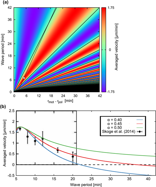
Figure 3. Averaged velocities for various parameter values. (a)Phase diagram of the averaged velocity (5) is shown. The color bar indicates the range of the averaged velocity. The horizontal axis represents the difference in the response times,  , and the vertical axis represents the wave period of the extracellular cAMP concentration, T. The solid line represents the critical wave period that satisfies
 ![${\rm sin} [2\pi ({{\tau }_{{\rm mot}}}-{{\tau }_{{\rm pol}}})/T]=0$](https://content.cld.iop.org/journals/1478-3975/12/2/026004/revision1/pb510555ieqn41.gif) , at which the direction of the net migration inverts. The filled white circle indicates the typical parameters at the aggregation state,
, at which the direction of the net migration inverts. The filled white circle indicates the typical parameters at the aggregation state,  min and T = 7 min, of D. discoideum (see table 1). The dashed line represents
  . (b) Averaged velocities (5) under the assumption,
 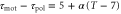 , for
, for  , 0.45, and 0.50 are shown with experimental data measured by Skoge et al (figure 1(E) (Lower) in [24]) with the permission of the corresponding author and PNAS.
Download figure:
Standard image High-resolution imageA recent study, in which motions of a cell under waves with several periods were investigated, allows us to estimate the dependence of the difference between the response times,  , on a wave period. We assume a linear dependence for simplicity and set it to
 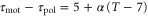 in order to satisfy
  when T = 7. Under this assumption, averaged velocities (5) for
  , 0.45, and 0.50 are obtained as figure 3(b). By comparing the averaged velocities with those measured by Skoge et al [24], we estimate α at 0.45. Using the linear dependence,
  , we obtain instantaneous velocities of a cell by numerically solving equation (1). Figure 4 shows the instantaneous velocities under the waves with the periods of 6, 10, and 16 min.
Figure 4. Instantaneous velocities for the periods of 6, 10, and 16 min.The blue, green and red lines are the instantaneous velocities of cells under the waves with the periods of 6, 10, and 16 min, respectively. (a) Instantaneous velocities obtained by the integration of equation (1) are shown as the function of the phase of the wave. We have used a sinusoidal waveform for S and the linear relation,  . Other parameters are given in table 1 except for
  and T. (b) Instantaneous velocities obtained by experiments by Skoge et al (figure 1(E) (Upper) in [24]) are shown with the permission of the corresponding author and PNAS.
Download figure:
Standard image High-resolution imageTo see that the essence of the result does not depend on the waveform, consider another situation in which the stimulation by the traveling wave of cAMP is sharply peaked and represented by

where S0 and S1 are positive constant parameters, and the chemotactic coefficient is given by equation (3). In the same manner as for the sinusoidal traveling wave, we ignore the periodic function and obtain

where  . We see that the direction of the net migration of the cell is determined by the sign of
 ![${\rm sin} [2\pi ({{\tau }_{{\rm mot}}}-{{\tau }_{{\rm pol}}})/T]$](https://content.cld.iop.org/journals/1478-3975/12/2/026004/revision1/pb510555ieqn54.gif) again.
again.
Even when the waveform of the cAMP is not as simple as in the above examples, as long as the waveform is periodic and mono-phasic, the wave period, T, and the difference between the two response times,  , are still key parameters governing the direction of the net migration. This is explained by a qualitative discussion in the following way.
Figures 5(a) and (b) illustrate two situations in which the wave periods, T, are different. Because the wave,  , is mono-phasic and periodic, the spatial gradient,
  , becomes a biphasic wave whose time average is 0. When the wave period is such that the peak of the motility,
  , appears while
  is positive in each cycle of the cAMP wave, the time average of the product of
  and
and  becomes positive (figure 5(a)). This result implies that the averaged velocity,
  , is positive, and the cell migrates toward the wave source (figure 5(a)). Conversely, when awave period is such that the peak of the motility
  appears when
  is negative in a cycle, the time average of the product of
  and
and  becomes negative (figure 5(b)). This result implies that the averaged velocity,
  , is negative, and the cell migrates away from the wave source (figure 5(b)). Thus, the wave period, T, determines the direction of cell migration.

Figure 5. Motion under waves with a short and long period. We show figures to qualitatively demonstrate the wave period dominates the net migration. The two response times are fixed as  min and
  min. From the top to bottom, the top five rows show the stimulation S(t), the polarity
  , the motility
  , the velocity v(t), and the position x(t). Each graph at the bottom is obtained by superimposing the graphs of the polarity, motility, and velocity and rescaling the gray region during one cycle of the waves in order to compare the phases in the oscillation of each quantity. (a) The wave period is 7 min. The cell migrates towards the wave source. (b) The wave period is 24 min. The cell migrates away from the wave source.
Download figure:
Standard image High-resolution imageFigures 6(a) and (b) illustrate two situations in which the differences between the two response times,  , are different. When two response times are such that the peak of the motility,
  , appears while
  is positive or negative in each cycle of the cAMP wave, the time average of the product of
  and
and  becomes positive or negative, respectively (figures 6(a) and (b)). Thus, the direction of the cell migration also depends on the difference between the two response times,
  .
.
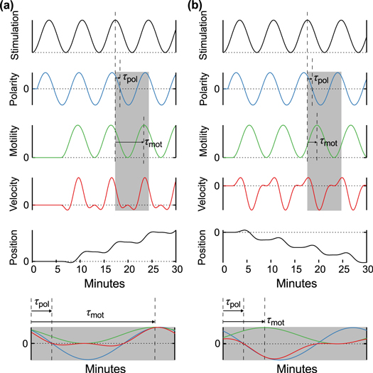
Figure 6. Motions with a small and large difference between the response times. We show figures to qualitatively demonstrate that the difference between the two response times dominates the net migration. The wave period is fixed as 7 min. From top to bottom, the top five rows show the stimulation S(t), the polarity  , the motility
  , the velocity v(t), and the position x(t). Each graph at the bottom is obtained by superimposing the graph of the polarity, motility, and velocity and rescaling the gray region during one cycle of the stimulus in order to compare the phases in the oscillation of each quantity. (a) The response times are
  min and
  min. A cell migrates towards the wave source. (b) The response times are
  min and
  min. A cell migrates away from the wave source.
Download figure:
Standard image High-resolution imageThe directional net migration of a cell has been reproduced in several models in which the time dependence of the chemotactic coefficient is taken into account [14–23]. We conclude that all of these models have been constructed in such a way that the appropriate phase difference between the stimulation and the response is generated.
3. Discussion
The above results are in good agreement with experimental results at four points. First, for the parameters in aggregation state(table 1), a cell migrates toward the wave source since the averaged velocity is positive, which explains the cell aggregation at the wave source. Second, as seen in figure 3(b), the averaged velocity (5) precisely describes experimental data over five different wave periods under an assumption of the linear dependence of the response times on wave periods,  . Third, as seen in figure 4, duration where the instantaneous velocity is obviously negative is reproduced. Note that the obvious negative velocity might not be explained by the adaptation mechanism [14–23] since a cell has been assumed to be stationary at the back of the wave in the mechanism. Fourth, two peaks in the instantaneous velocities during one wave period experimentally observed are also found in the theoretical results as seen in figure 4. This characteristic is remarkable in terms of mathematics because it indicates that the instantaneous velocity has a sinusoidal component whose period is
  . The present model has this component as we see in equation (4). It is produced by the multiplication of two sinusoidal functions, χ and
  , both of whose periods are T. While these consistencies with experiments exist, the instantaneous velocities are not precisely reproduced (figure 4). In particular, the memory effect found in [24], that is the tendency to keep the migration direction, is not well described. This might be because the relaxation of the motion is not considered in the present model.
The present results suggest that cAMP also plays a role as a 'chemorepellent.' Conventionally, when a cell migrates away from the source of a chemical signal, the signal has been referred to as a chemorepellent [38, 39]. However, we have found that even if the signal is composed of the chemoattractant, the cell moves both toward and away from the wave source depending on the wave period. According to figure 3(a), if the wave period is sufficiently large, a cell should move away from the wave source. The critical wave period at which the direction of the net migration inverts is estimated at 37 min, which is calculated from 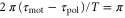 and
and  . In particular, the cell migrates away from the wave source when it is exposed to a single pulse as far as
  (see appendix
According to figure 3, when the period of the cAMP wave is less than a couple of minute, the speed and direction of the net migration of a cell would be very sensitive to two response times,  and
and  . However, this model would not be suitable for predicting the motion of a cell under a wave or stimulation with so short periods [40, 41] because the present model does not incorporate all cellular processes that have a time scale smaller than
  min.
min.
The emergence of the directional net migration discussed here is understood as an example of spontaneous breakage of symmetry in biology. The specific direction in which a cell migrates on average is determined from the nondirectional periodic change in the concentration and gradient of cAMP. Thus, the coupling of the two nondirectional periodic stimulations produces net migration in a particular direction.
Acknowledgments
The authors would like to thank Prof Dan Tanaka and Prof Yuki Sugiyama for fruitful discussions, and a referee for pointing out the work of Skoge et al [24], and Prof Rappel and PNAS for the permission of the use of figure 1(E) in [24]. This work was supported by JSPS KAKENHI Grant Number 26800208.
Appendix A.: Derivation of the model equation
The following theoretical analysis indicates that the equation of motion for chemotactic cells should be formulated as the product of the chemotactic coefficient, χ, and gradient of cAMP,  . The equation of motion for the cell is generally formulated as,

as long as we neglect the inertial effect of the cell. Here, F denotes external forces, ξ denotes the force that induces random motion of the cell [42, 43], and the coefficient γ is referred to as the friction coefficient. The equation reads,

In the absence of the spatial gradient of the cAMP and other external forces, the equation (A.2) is reduced to

According to the experiments performed by Soll et al [16, 25–27], the temporally periodic and spatially uniform stimulation by cAMP induces a periodic response of instantaneous velocity with a constant response time with the same period. Here, we attribute the oscillation of the velocity to the oscillation of  . Additionally, when a cell is exposed to a traveling wave of the signal of cAMP, S, the F is proportional to the gradient
  , that is,

Omitting the random component ξ because we are not interested in the detailed motion of each cell, equation (A.1) is reduced to

where the chemotactic coefficient, χ, is proportional to  .
.
Appendix B.: Derivation of equation (4)
Substituting equations (2) and (3) into the equation of motion (1), we obtain

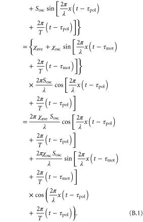
We can generate the approximations  and
and 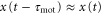 because the velocity of the traveling wave is much greater than the speed of the cell [9, 34]. Then, the equation of motion is reduced to

Using the trigonometric addition formula,  , we rewrite equation (B.2) into

Thus, we obtain equation (4).
Appendix C.: Motion of a cell for pulsatile stimulation
Figure C1 shows the result of the numerical simulation of the motion of a cell under a single sharply peaked pulse. We use typical parameter values in the aggregation process given in table 1. As a result, the cell migrates away from the wave source under the single sharply peaked pulse.

Figure C1. Numerical simulation of the motion of a single cell under a sharp cAMP pulse. The cell migrates away from the wave source under the single sharply peaked pulse.
Download figure:
Standard image High-resolution image
Whenever two response times satisfy  , because the peak of the motility
  appears when
  is negative, the product of
  and
and  becomes negative.