

Abstract
Quantum metrology offers significant improvements in several quantum technologies. In this work, we propose a Gaussian quantum metrology protocol assisted by initial position-momentum correlations (PM). We employ a correlated Gaussian wave packet as a probe to examine the dynamics of Quantum Fisher Information (QFI) and purity based on PM correlations to demonstrate how to estimate the PM correlations and, more importantly, to unlock its potential applications such as a resource to enhance quantum thermometry. In the low-temperature regime, we find an improvement in the thermometry of the surrounding environment when the original system exhibits a non-null initial correlation (correlated Gaussian state). In addition, we explore the connection between the loss of purity and the gain in QFI during the process of estimating the effective environment coupling and its effective temperature.

Original content from this work may be used under the terms of the Creative Commons Attribution 4.0 licence. Any further distribution of this work must maintain attribution to the author(s) and the title of the work, journal citation and DOI.
1. Introduction
The search for optimal measurement of properties during classical or quantum noisy processes i.e. determining the ultimate precision in which a parameter can be estimated, after eliminating all technical noise, using ideally accurate instruments, and repeatedly preparing the system in the same state, is crucial for the development of quantum technologies [1]. Quantum metrology offers significant applications such as superresolution imaging [2], high-precision clocks [3], estimation of proper times and accelerations in quantum field theory [4], navigation devices [5], magnetometry [6], optical and gravitational-wave interferometry [7, 8], and thermometry [9].
Currently, the capacity to measure low temperatures accurately in quantum systems is important in a wide range of proof of principles experiments. It has attracted significant interest recently due to its critical role in optimizing the performance of quantum technologies [10, 11]. For instance, effective two-level atoms can be employed to minimize the undesired disturbance on the sample, and an optimum quantum probe (a small controllable quantum system) can act as a thermometer with maximal thermal sensitivity [12]. The scaling of the temperature estimation precision with the number of quantum probes was investigated [13], and the impact of initial system-environment correlations was examined to enhance the estimation of environment parameters within the spin-spin model at low temperatures [14]. Still in the low-temperature limit, as a fundamental aspect of the third law of thermodynamics, the unattainability principle of reaching absolute zero also implies the impossibility of precisely measuring temperatures near absolute zero [15–17]. A general approach to low-temperature quantum thermometry considers restrictions from both the sample and the measurement process [15]. In continuous-variable systems, a non-Markovian quantum thermometer was proposed to measure the temperature of a quantum reservoir, effectively avoiding error divergence in low temperatures [18]. Optimizing the interaction time in a bipartite Gaussian state also allows for precise estimation of the local temperature of trapped ions [19].
Employing quantum resources such as coherence and entanglement, it is possible to improve, until the Heisenberg limit (HL), the measurement precision beyond the classical shot-noise limit [20–22]. Recently, it was presented a method for low-temperature measurement that improves thermal range and sensitivity by generating quantum coherence in a thermometer probe [23]. Optimal quantum metrology strategies usually employ entanglement in initialization and readout stages to significantly enhance measurement precision [24, 25]. However, producing entangled states or measurements with high precision in high-dimensional or continuous-variable systems is not a trivial task. Relatively small errors are known to ruin the success of such tasks compared to the optimal classical one, and implementing a hybrid quantum-classical approach to automatically optimize the controls has been taken into consideration [26].
In this work, we employ a position-momentum (PM) correlated Gaussian state in quantum metrology. To work with it, a real parameter can be controlled such that when it is null, the state recovers the standard uncorrelated Gaussian wave packet form. PM correlations were originally investigated by considering the quantized operators and , with [27]. These correlations generalize Glauber's coherent states [28, 29] and minimize the Robertson-Schrödinger uncertainty relation. Practically, this parameter arises from atomic beam propagation along a transverse harmonic potential, acting as a thin lens and causing a quadratic phase shift in the initial state [30]. Gaussian correlated packets have applications in various fields, including quantum optics and double-slit matter-wave interferometers [31–35]. However, practical applications face challenges due to errors in tuning the parameter, caused by non-ideal incoherent sources of matter waves and the focalization method used to produce it [36–38].


![$[\hat{x},\hat{p}]=i\hslash $](https://content.cld.iop.org/journals/1402-4896/100/1/015111/revision2/psad9a18ieqn3.gif)
Here, we propose a scheme to estimate PM correlations. Our protocol consists of three stages, initialization, interaction, and estimation. Moreover, we further apply our protocol to estimate the effective environment coupling and its temperature (thermometry), and we show that the correlated Gaussian system can outperform the standard (uncorrelated) one. More specifically, we estimated the effective temperature of a Markovian bath via the environmental coupling with our quantum thermometer based on a single-mode correlated Gaussian system. Such correlations impact the Quantum Fisher Information (QFI) after the evolution of the initial state through a Markovian bath and establish the conditions to improve our quantum thermometer model assisted by PM correlations.
The dynamics of the QFI and purity will be analyzed to better estimate this initial position-momentum correlation using the Classical Fisher Information (CFI). Purity, like other measures such as entanglement [39], quantum discord [40–42], and quantum coherence [43], is also a resource, where it is quantified by deviations from the maximally mixed state [22, 39, 43–48]. Purity can be operationally interpreted as the maximum coherence achievable by unitary operations [48]. It bounds the maximum amount of entanglement and quantum discord that unitary operations can generate, acting then as a fundamental resource for quantum information processing [48]. Unlike other measures, purity is easily accessible in experiments, providing experimental bounds to other quantum quantifiers [49–51]. In the following, we present our main results. First, we describe our general estimation protocol in section 2.1. Then, we investigate the noise environmental effect on PM correlations estimation in section 2.2. Finally, in section 2.3 we analyze the role of PM correlation in improving the thermal sensitivity in the low-temperature regime, and in section 3 we discuss our results.
2. Results
2.1. Estimation protocol
Our quantum estimation protocol schematized in figure 1 is represented in three parts: initialization, interaction, and estimation. The initialization step is characterized by the generation of fullerene Gaussian wave packets with momentum and an initial coherent length ℓ0. In the sequence, the parameterization process of unknown parameters is separated into two parts. The first one, here denoted as focalization, describes the unitary parameterization associated with the encoding of the PM correlation parameter γ employing a real-noisy source (details about this process are discussed in appendix B). The second one, denoted as interaction, represents a non-unitary parameterization for which the probe interacts with a Markovian bath producing an encoding of the effective environment coupling parameter Λ and in turn its temperature T in the correlated Gaussian state. Finally, the estimation procedure of the unknown parameters is carried out during the estimation stage. This stage includes (I) PM correlations and (II) thermometry estimations.


Figure 1. Theoretical protocol to describe the estimation of the parameters γ (PM correlations) and Λ (effective environmental coupling). The initialization step is the source production of fullerene wave packets with momentum and initial coherent length ℓ0. Then, the focalization step takes place, generating the initial position-momentum correlations γ (see appendix B). After, the system interacts with the Markovian thermal bath, characterized by the effective environmental coupling Λ. In the readout stage, parameter estimations are done.

Download figure:
Standard image High-resolution imageWe consider as the initial state the following correlated Gaussian state of transverse width σ0

that represents a PM-correlated Gaussian state [52]. The real parameter γ ensures that the initial state is correlated [52, 53]. Considering the initial state, equation (1), the variance in position becomes , whereas the variance in momentum is , and the initial correlations PM is . Notice that, for γ = 0 we have a simple uncorrelated Gaussian wave packet, i.e. σxp = 0. Exploring the Pearson correlation coefficient between and , i.e. , the γ parameter turns out to be , illustrating the physical meaning of the γ as a parameter that encoded the initial correlations between position and momentum for the initial state.


In the standard quantum phase estimation protocols, it is usual to estimate the physical parameter that implements a relative phase shift [54, 55]. Here, our main goal will be to explore whether initial PM correlations can work as a resource to improve quantum metrology under noise. To estimate the initial PM correlations, we consider the production of beam particles from a non-ideal or partially incoherent source (see figure 1), where each particle has momentum px = ℏkx in the x-direction within a certain range of wavenumber kx and can be modeled by the following initial density matrix [37, 56, 57]


with . In this model, we consider wave effects only in the x-direction since the energy associated with the momentum of the particles in the z-direction is high enough such that the momentum component pz is sharply defined, i.e. Δpz ≪ pz. Then, the behavior in the z-direction can be considered classical [37]. The geometry of the collimation device is such that it selects only particles with a transverse wave number kx inside a specific range defined by the width σkx, being described by a classical Maxwell–Boltzmann distribution, . After some algebraic modifications, the initial density matrix of the coherent correlated Gaussian wave packet becomes


where , , , , and is related with the coherence level of the initial state. It is important to note that, in the limit σkx → 0 (ideal collimation), one has ℓ0 → ∞ (), meaning that the initial state (3) is completely coherent or pure. On the other hand, if σkx → ∞, then one has ℓ0 → 0 (), indicating a completely incoherent or mixed state.


According to the protocol depicted in figure 1, after the focalization process, the system interacts with an environment that is considered to be a Markovian bath [58], and its evolution is given by

where

is the propagator which includes the environmental effect [37, 59]. We consider the propagation of fullerene molecules and the decoherence effect produced by air molecules scattering [37]. In this case, the effective scattering constant is given by , where N is the total number density of the air, mair is the mass of the air molecule, w is the size of the molecule of the quantum system, kB is the Boltzmann constant, and T is the bath temperature [59]. In the propagator described by equation (5), it is assumed that the center-of-mass state of the system remains undisturbed by the scattering events, a valid condition for fullerene molecules (m ≫ mair) [37]. The environmental scattering decoherence is a ubiquitous effect constantly monitoring the position of quantum systems in the cosmos, that can be caused by air molecules, light (optical photons), solar neutrinos, cosmic muons, background radioactivity, and even the Universe's 3 K cosmic background radiation [59]. It is also essential to emphasize that in the derivation of this model, it was also assumed the following conditions [59, 60]: the system and the surroundings are not initially correlated; when the composite object–environment system is translated, the scattering interaction remains unchanged; the rate of scattering is much faster than the characteristic rate of change in the state of the system; and the distribution of momenta of the particles in the environment is isotropic and obeys a Maxwell–Boltzmann distribution. In physical terms, the Λ parameter quantifies the rate at which spatial coherence over a given distance Δx is suppressed, motivating the introduction of a decoherence timescale given by [59]


This equation will be useful for interpreting how PM correlation is related to loss of purity and gain of Fisher information. After integration and manipulating equation (4), we get

where , , and are parameters that include the interaction with the Markovian bath (see appendix C).


Employing equation (7), we can cast the purity of the state in the concise form
![$\mu (\gamma ,{\rm{\Lambda }},t)=\,\rm{tr}\,\left[{\rho }_{{\rm{\Lambda }}}^{2}(x,{x}^{{\prime} },t)\right]$](https://content.cld.iop.org/journals/1402-4896/100/1/015111/revision2/psad9a18ieqn28.gif)

where , and . This result produces μ = 1 when ℓ0 → ∞ (), i.e. for a completely coherent source and no environment effect Λ = 0. Outside this regime, we always have μ(γ, Λ, t) < 1, typical of a noisy scenario represented by mixed states (details in appendix C).
![${{ \mathcal A }}_{R}=\,\rm{Re}\,[{{ \mathcal A }}_{t}]$](https://content.cld.iop.org/journals/1402-4896/100/1/015111/revision2/psad9a18ieqn29.gif)
![${{ \mathcal B }}_{R}=\,\rm{Re}\,[{{ \mathcal A }}_{t}]$](https://content.cld.iop.org/journals/1402-4896/100/1/015111/revision2/psad9a18ieqn30.gif)
![${{ \mathcal C }}_{R}=\,\rm{Re}\,[{{ \mathcal A }}_{t}]$](https://content.cld.iop.org/journals/1402-4896/100/1/015111/revision2/psad9a18ieqn31.gif)

In the following subsections, we present the dynamics of the QFI and the purity in each part of the parameterization process illustrated in our estimating protocol in figure 1. We begin estimating PM correlations in a scenery where the quantum system unavoidably interacts with its surrounding environments and then we explore how these correlations can enhance noisy quantum metrology.
2.2. PM correlations estimation
From the mixed Gaussian state described in equation (7), it is easy to check that the first moments are null and the dimensionless second moments are given by


Here, is the time at which the distance of the order of the wave packet extension is traversed with speed corresponding to the dispersion in velocity [61]. Then, the covariance matrix σ and its inverse σ−1 can be written as


where σpx = σxp, adj(σ) is the adjugate matrix of σ and we have used that, for Gaussian states, det(σ) = μ−2 [62]. The mean number of excitations, which is proportional to the energy of the system, can then be expressed for the single-mode system as follows [63]:

In optics, the quantity n represents the mean photon number. This quantity will be important to analyze how the QFI scales with n, allowing a comparison with the shot noise and the Heisenberg limit (HL), more details in figure.
Therefore, we can write the QFI for single-mode Gaussian states (see equation (A5) in appendix A) as following [64, 65]

The above expression will be useful for interpreting our results, where we can explicitly understand the role of purity and its derivative as a resource for estimating unknown parameters in the presence of noise. Furthermore, we also investigate the dynamics of Classical Fisher Information (CFI) obtained from the density distribution in position space as

where . In what follows, the estimated parameters will be the initial position-momentum correlation Θ = γ and the effective environmental coupling constant Θ = Λ.

We employ the QFI and CFI for the estimation of the initial correlations. They were calculated from equations (13) and (14) by making Θ = γ. After some simplifications, we obtain

and

where the parameter B is explicitly defined in appendix C and Φγ(γ, t, Λ) is a monotonic increasing function of the parameters γ, t and Λ (see appendix D). Since this function is multiplied by the fourth power of μ, the purity behavior determines the first term in QFI. This can be illustrated using the following parameters: fullerene mass m = 1.2 × 10⁻²⁴ kg, molecular size w = 7 Å, the width of the initial wave packet σ0 = 7.8 nm, the mass of the air molecule mair = 5.0 × 10⁻²⁶ kg and density of the air molecules N = 1012 molecules/m3[37, 38, 56]. It is assumed that the collimator apparatus selects wave numbers in the Ox direction, with a transverse wavenumber dispersion of . This corresponds to an initial coherence length of . Parameters of this order of magnitude were previously used in experiments with fullerene molecules by Zeilinger [66, 67]. With the other parameters fixed, the variation in Λ corresponds to the variation in the environmental temperature such that, Λ ∝ T3/2. For instance, Λ of the order of 1019 m−2s−1, corresponds to an effective temperature around 205 K. The value 3.2 × 10¹⁵ m−2s−1 for the scattering by air molecules estimated in [37] for the experiment with fullerene molecules corresponds to a temperature of 300 K and a density of the air molecules of N = 1.8 × 10⁸ molecules/m3, smaller than the densities we are considering. In other words, the air molecule density and temperature range we are exploring here are experimentally feasible with the current technology.


To analyze the role of each term in the QFI (13) and the influence of the environmental effect, we present in figure 2 the behavior of the QFI (), CFI (), purity μ, and its absolute relative derivative as a function of the initial correlation γ for a characteristic interaction time t = 1.0μs and different environmental effect coupling constants. Panels (a) and (b) demonstrate that the QFI behaves similarly to the purity when the environment has a relatively small effect (low-temperature regime). In contrast, panels (c) and (d) demonstrate that the QFI behaves according to the absolute purity variation when the environment effect is stronger. Also, we see that only in the regime of strong environmental effect (quantum to classical transition in the high-temperature regime) does the CFI become comparable with the QFI.


Figure 2. Curves for QFI (), CFI (), purity μ, and its absolute relative derivative as a function of the initial correlation γ for t = 1.0μs, and crescents environmental effect coupling constants: (a) Λ = 0 (T = 0 K), (b) Λ = 1020 m−2s−1 (T = 952 K), (c) Λ = 1022 m−2s−1 (T = 20.5 × 10³ K), and (d) Λ = 1023 m−2s−1 (T = 95.2 × 10³ K). In panels (a) and (b), we observe that when the environment has a small effect (low-temperature regime), the QFI exhibits a behavior similar to the purity. In contrast, panels (c) and (d) show that the QFI exhibits a behavior related to the absolute purity variation when the environment has a strong effect (high-temperature regime). The advantage of employing PM correlations can be realized for small values of purity.


Download figure:
Standard image High-resolution imageOne of the most intriguing features here is that besides the suppression of the QFI when the noise increases, we can find PM correlations that enhance the corresponding QFI compared to the usual Gaussian state. It is also important to note that figure 2(d) shows that even a maximal purity value (corresponding to a null PM correlation) does not provide the maximum value for the QFI. This happens because, in the regime of strong environmental effect, the change in purity (second term in equation (15)) is dominant over the purity value itself is close to zero, and will be elevated to the fourth power (first term in equation (15)). To comprehend in more detail how the QFI behavior is governed by either the purity or by the purity variation, and how this transition occurs, we present in appendix D these quantities where we fixed Λ and plotted them as a function of the PM correlations and the propagation time.
2.3. Quantum thermometry assisted by PM correlations
Here, we analyze how the PM correlations affect the estimation of the effective environmental coupling constant, showing a specific regime in which the correlated Gaussian state provides a quantum advantage over the standard one in estimating the effective parameter related to an environmental interaction. Using equations (13) and (14) and setting Θ = Λ, the QFI and CFI reads

and

where ΦΛ(γ, t, Λ) is another monotonic increasing function of the parameters γ, t and Λ (see appendix E). Similarly, this function does not determine the profile of QFI in the first term.
In figure 3, we exhibit the curves for QFI (), CFI (), purity μ, and its absolute relative variation as a function of initial correlation γ for t = 50.0μs and considering (a) weak environmental effect (Λ = 1.0 × 10¹⁵ m−2s−1 or T = 442 mK) and (b) strong environmental effect (Λ = 1.0 × 10²¹ m−2s−1 or T = 4.4 × 10³ K). Again, we observe two characteristic regimes, the gain in QFI is related either to purity or relative variation in purity when the environmental effect is strong (high-temperature regime) or weak (low-temperature regime), respectively. Such regimes are associated with the first and second term in equation (17), respectively. One of the more interesting results of this work, rarely explored in the literature, is investigating the relation between loss of purity and gain in Fisher information. Also, we can observe that in the low-temperature regime, the PM can improve the QFI, and this behavior paves the way for exploring the enhancement of noisy quantum metrology by PM correlations which will be discussed in the following. On the other hand, these PM correlations quantum advantage ceases to be valid in the limit of strong environmental effect (Λ = 1.0 × 10²¹ m−2s−1 or T = 4.4 × 10³ K), with the standard uncorrelated Gaussian state γ = 0 providing the best sensitivity for thermometry in this regime [see figure 3 (b)].


Figure 3. Curves for QFI (), CFI (), purity μ, and its absolute relative variation as a function of initial correlation γ for t = 50.0μs and considering (a) weak environmental effect (Λ = 1.0 × 10¹⁵ m−2s−1 or T = 442 mK) and (b) strong environmental effect (Λ = 1.0 × 10²¹ m−2s−1 or T = 4.4 × 10³ K). We observe in panel (b) [(a)] that the gain in Fisher information is related to purity (relative variation in purity) when the environmental effect is strong (weak).


Download figure:
Standard image High-resolution imageAlso, it is important to mention that the effect of increasing the interaction time t or changing the environmental effect Λ is almost equivalent from a theoretical point of view, they both decrease the purity and coherence of the quantum state. However, from an experimental point of view, the variation of these two parameters is very different. The first is varied just by moving the position of the detector to regions further away from the source. In contrast, the second can be varied by changing, for example, the environmental temperature or the air pressure.
In figure 4 we investigate the time dependence of (a) QFI () and (b) purity μ for different values of the initial correlation γ and considering Λ = 1.0 × 10¹⁵ m−2s−1 (T = 442 mK). We observe a temporal quantum enhancement due to PM correlation γ. Therefore, employing an initial correlated (position-momentum) Gaussian state can reduce the time required to obtain the maximum amount of information until it is saturated. Moreover, note the relationship [inset of panel (b)] between the maximum temporal rate of purity variations and the time of information saturation. We interpret this gain in QFI as being associated with the rate of change of purity. This relationship can be seen directly through the inset in figure 4 (b), showing that for large times and regardless of the value of γ the second term in equation (17) ceases to contribute to an increase in QFI since purity goes to zero at this limit. In other words, the second term contributes to an enhancement in the QFI only up to approximately 300 microseconds, during which the presence of PM-correlations can further improve this gain. In this context, a similar effect was recently observed in [68], where it was noted that the rate of change of coherence concerning the channel parameter—rather than the amount of coherence—can produce a parameter estimation gain.


Figure 4. (a) QFI () and (b) purity μ as a function of time t and for different values of the initial correlation γ and considering Λ = 1.0 × 10¹⁵ m−2s−1 (T = 442 mK). We can observe a quantum enhancement due to γ. Also, note the relation exists between the time of information saturation and the correspondent maximum temporal rate of purity variation [inset of panel(b)].

Download figure:
Standard image High-resolution imageBesides this, to quantify such an enhancement or acceleration in the time required to saturate the QFI due to PM correlation γ, we introduce the Temporal Gain of Information (TGI), defining it on the decibel scale as follows

where the time τmax corresponds to the maximization point of the relative purity variation, i.e. the maximum of [see inset of figure 4(b)]. In this definition, the acceleration in the time to saturate the QFI is compared with the correspondent time needed for the standard uncorrelated Gaussian state (γ = 0), such that the uncorrelated state is always associated with a null temporal gain.

To obtain a simplified and closed expression for the TGI as a function of PM correlations γ, we consider interaction times in the order of some microsecond and since the cubic term in equation (C5) becomes dominant, and therefore the purity can be approximately expressed as


Then, the time τmax that maximizes the relative purity variation, i.e. the maximization point of is given by


Note that this time can be reduced by increasing the initial correlation γ. In this way, using τmax(Λ, γ) from equation (21), the approximate TGI(γ) can be written explicitly as

In figure 5, we examine the enhancement in TGI as a function of PM correlation γ. The solid red line corresponds to the approximate gain calculated from equation (22). The full circles correspond to particular TGI values determined by a precise number that optimizes the function without any approximation in the purity expression. These points are obtained directly by probe inspection in the inset of figure 4(b) and are summarized in table 1. Moreover, this procedure was applied to obtain an approximate and simple expression for the TGI and its dependence on the PM correlations γ. Note that for PM correlation on the order of 150, the gain achievable is almost 15 dB over the standard uncorrelated Gaussian state. In experimental terms, this parameter can be controlled, for example, by changing the laser frequency or intensity in the initialization step (see appendix B).


Figure 5. Temporal Gain of Information (TGI) as a function of initial PM correlation γ. The solid red line corresponds to the approximate gain calculated from equation (22). The full circles correspond to some values of TGI obtained from the exact value that maximizes the function without any approximation in the purity expression. These points are summarized in table 1.

Download figure:
Standard image High-resolution imageTable 1. Values with the time improvement in the estimation environmental effect for Λ = 1015 m−2s−1.
| γ | τmax (μs) | μ(τmax) | (s−1) | TGI (dB) | |
|---|---|---|---|---|---|
| −50.0 | 17.1 | 0.563 | 58 488 | 0.246 | 11.28 |
| −25.0 | 27.2 | 0.563 | 36 861 | 0.247 | 9.24 |
| −1.0 | 183.2 | 0.563 | 5 472 | 0.247 | 0.97 |
| 0.0 | 228.4 | 0.563 | 4 377 | 0.247 | 0 |
| 35.0 | 21.7 | 0.563 | 46 117 | 0.247 | 10.22 |
| 70.0 | 13.7 | 0.563 | 73 191 | 0.248 | 12.23 |
| 150.0 | 8.2 | 0.563 | 121 646 | 0.247 | 14.45 |


The quantum Cramér-Rao bound often provides a generalized uncertainty relation, even if no Hermitian operator can be simply associated with a given observable [69], as is the case, for phase estimation. In this context, the vacuum fluctuation (shot noise) imposes that one can estimate the phase values with a statistical error ΔΘ proportional to , using a classical beam with n average photons or n separate single-photon beams. However, it has been shown that the injection of a squeezed vacuum into the typically unutilized port of an interferometer enables the attainment of a sensitivity of 1/n3/4 [70]. Conversely, sensitivity can be further enhanced by employing entangled states, resulting in a resolution that scales inversely with n, thereby achieving the Heisenberg limit (HL). To investigate the scaling of the QFI with n and compare the quantum advantage provided by PM correlations against shot noise, squeezing, and the Heisenberg limit, we exhibit in figure 6 the QFI () dependence with the mean number of excitations n in log scale for different values of the initial correlation γ and considering Λ = 1.0 × 10¹⁵ m−2s−1 (T = 442 mK). The solid straight lines correspond to a power law fitting of the form , where s adjusts how the Fisher scales with n. This plot was generated in part from figure 4, in terms of temporal parameterization t of the QFI behavior and the mean number of excitations n [see equation (12)]. In the context of statistical error and using the Cramér-Rao inequality (A2), it can be observed that the sensitivity in estimating the effective environmental coupling constant Λ scales as 1/n(1+s)/2. The values s = 0 (s = 1) correspond to the shot noise limit (HL), respectively, while s = 1/2 to the sensitivity of a squeezed vacuum state in a closed quantum system. Thus, the value of s ≈ 0.2 for γ = 70 indicates a dependence of 1/n0.6, demonstrating that PM correlations can be applied to beat the shot noise limit and is almost close to the squeezing dependence of 1/n0.75 (see also appendix F where we explore the connection of PM correlation with squeezing), but is still relatively far from reaching HL. Since the generation of entanglement is typically a resource-intensive process, this finding is particularly relevant, as it suggests the potential for metrological enhancement solely through the correlation between two degrees of freedom associated with conjugate observables. This paves the way for advancing quantum metrology without requiring resources like entanglement.


Figure 6. QFI () dependence with the mean number of excitations n in log scale for different values of the initial correlation γ and considering Λ = 1.0 × 10¹⁵ m−2s−1 (T = 442 mK). The solid straight lines correspond to a power law fitting of the form , where s adjust how the Fisher scales with the mean number of excitations n. We can observe an enhancement in how the QFI scales with n due to γ.


Download figure:
Standard image High-resolution image3. Discussion
Concepts such as purity distillation and purity cost, analogous to entanglement distillation and entanglement cost, were introduced to quantify this resource [71, 72]. Transformations from pure to mixed states are usually associated with information loss and irreversibility [71]. However, this work explores the relationship between Quantum Fisher Information (QFI) and purity rate, focusing on a regime where purity loss primarily drives QFI behavior. It examines how position-momentum (PM) correlated probes can enhance noisy quantum metrology of the environmental thermal bath and demonstrates that PM-correlated Gaussian states can outperform standard uncorrelated Gaussian states in estimating the effective environmental coupling constant.
We started presenting the probe initialization procedure and how the PM correlation can be controlled and produced at this stage. We then calculated the dynamics of QFI and purity for the probe as it evolves through a decoherence channel, representing the scattering model, one of the most common sources of decoherence in physical systems [59, 60]. This decoherence model describes how the entanglement of the system with the environmental particles (fermionic or bosonic bath), caused by countless scattering events, delocalizes local phase relations between spatially separated wave-function components, leading to decoherence in position space (i.e. to localization) [59]. Our findings demonstrate the role of purity and purity 'velocity' (∂Θμ) as a resource for estimating unknown parameters in the presence of noise [see equation (13)].
We observed that, in estimating the PM correlation, when the decoherence factor is relatively small (i.e. low-temperature regime), the QFI and purity curves have similar behaviors. However, for high temperatures, the QFI is dependent on the rate of change of purity. In this configuration, maximum purity does not necessarily imply maximum values for the QFI due to the dynamics of the purity rate of change term for regimes with an effective strong coupling with the Markovian bath. As expected, QFI tends to match CFI under conditions of quantum-classical transition (high-temperature regime). Furthermore, we found scenarios where the QFI can be asymptotically estimated by the value of CFI by a suitable preparation of the correlated γ initial state [see, for example, figure 2(a)]. From a practical standpoint, this result is both surprising and useful, since obtaining the QFI is challenging because it requires maximizing all possible POVMs to ensure that estimations are independent of the chosen POVM and to achieve optimal measurement precision.
Regarding the estimation of the effective environmental coupling constant, we observed an improvement in the thermometry of the surrounding environment when the probe was prepared in a non-null initial correlated Gaussian state. Specifically, in this part, we explored the acceleration in the loss of purity, due to correlations, as a resource for increasing the QFI [second term in equation (17)]. Once the parameter Λ quantifies the decrease rate in spatial coherence, and since PM correlation values imply that high momentum values are correlated with high spatial values, as a result, we have an extended wavepacket for the probe state. This consequently causes an increase in the decoherence rate [see equation (6)], reducing the purity of the state. In our model, we considered the long-wavelength limit [59], where the wavelengths of scattering air molecules are much longer than the wave packet extension of the probe. Consequently, a large number of scattering events are needed to resolve the fullerene position by encoding substantial which-path information in the environment, ensuring weak coupling and resulting in an effective Markovian bath. Once we consider that the momentum of environment particles obeys a Maxwell–Boltzmann distribution, the temperature regime investigated here is still more than one million times greater than the ultra-low temperatures obtained, for example, in a Bose-Einstein condensate on the order of 170 nK [73]. Similarly, for example, the amplitude-damping channel [74], which models physical processes such as spontaneous emission, occurs at T = 0 K, and even so, Markovianity is maintained since the coupling of the system with the infinite vacuum modes is weak.

The findings discussed here can be extended to more general scenarios. For instance, recently it was shown that incorporating additional degrees of freedom in molecules, such as rotations and vibrations, can significantly enhance sensitivity when using molecular sensors as probes [75, 76], creating new opportunities for their application in quantum protocols. Building on this, one could integrate these degrees of freedom into our estimation protocol to fully explore the advantages of molecular probes. Additionally, our findings could also be expanded to include more complex dynamics through a generalized channel that accounts for non-Markovian memory processes. This would offer deeper insights into non-Markovian decoherence features in structured reservoirs, such as decoherence-free states [77]. By pursuing this approach, one could also advance in the exploration at even lower temperatures by relaxing the Born-Markov approximation [18, 78].
In conclusion, the observation that metrological enhancement can be achieved through the correlation of two degrees of freedom associated with conjugate observables is particularly noteworthy, especially considering the typically resource-intensive nature of generating entanglement. This finding paves the way for new explorations in quantum metrology that do not depend on entanglement, indicating a promising direction for future research.
Acknowledgments
J. C. P. Porto acknowledges Fundação de Amparo à Pesquisa do Estado do Piauì (FAPEPI) for financial support. L.S.M. acknowledges the Federal University of Piauì for providing the workspace. P.R.D acknowledges support from the NCN Poland, ChistEra-2023/05/Y/ST2/00005 under the project Modern Device Independent Cryptography (MoDIC). I.G.P. acknowledges Grant No. 306528/2023-1 from CNPq. C.H.S.V acknowledges the São Paulo Research Foundation (FAPESP), Grant. No. 2023/13362-0, for financial support and the Federal University of ABC (UFABC) to provide the workspace.
Data availability statement
All data that support the findings of this study are included within the article (and any supplementary files).
Appendix A.: Fisher information
Here, we review the definitions and differences between classical and quantum Fisher information, as well as the definition of purity and its relation to resource theory. Our focus is on describing valid relations specifically for Gaussian states.
A.1. Classical fisher information
The Fisher information is a measure of information that an observable random variable carries about an unknown parameter [79]. It expresses the level of uncertainty of a measured physical quantity. Let P(xi∣Θ) be the conditioned probability of measuring data xi given a specific value of Θ. The Classical Fisher Information (CFI) for estimation of the parameter Θ is defined by

If P(xi∣Θ) exhibits a peak as a response to variations in Θ, then, the data xi provides the information needed to estimate the parameter Θ. On the other hand, when P(xi∣Θ) is flat, numerous samples of xi would be required to estimate the value of Θ, which would be determined only by using the complete sample population. In this context, the Cramér-Rao inequality [80] establishes the lower bound on standard deviation of the estimated parameter


where n is the number of times that the experiment is repeated. Therefore, the Fisher information determines the reachable accuracy of the estimated quantity and represents the figure of merit in parameter estimation problems. Import to mention, that this inequality is valid only for unbiased estimators, i.e. estimators for which 〈Θest〉 = Θreal.
In quantum theory, we use a set of positive operator-values measure (POVM) , parameterized by κ, to describe the measurement procedure. These operators are positive and satisfy to ensure normalization. The probability can be expressed as . Using P(κ∣Θ) as the probability distribution, the CFI is defined as


![$P(\kappa | {\rm{\Theta }})=\,\rm{Tr}\,[\hat{\rho }\{\hat{A}(\kappa )\}]$](https://content.cld.iop.org/journals/1402-4896/100/1/015111/revision2/psad9a18ieqn68.gif)

where is the density operator describing the system. Naturally, optimal POVMs are those characterized by a statistical distribution of measurement results that is maximally sensitive to changes in the parameter Θ [81].

A.2. Quantum fisher information
The Quantum Fisher information (QFI), here denoted by , is defined by maximizing equation (A3) over all possible POVMs as follows [82–85]


The quantum estimation is then related to the optimal possible measurement precision. Note that this maximization procedure turns the QFI into an upper bound for the classical one, i.e. [84]. Quantum metrology is not the only application of quantum Fisher information, alternatives include quantum cloning [86], entanglement detection [87, 88], and quantum phase transition [89]. Feng and Wei [90] have highlighted the relationship between quantum coherence and Quantum Fisher Information (QFI), demonstrating that QFI is useful for quantifying quantum coherence. This relationship is established because QFI satisfies monotonicity under typical incoherent operations and convexity when quantum states are mixed. In [91], it was demonstrated how QFI can be used to identify quantum correlations such as steering, showing that such correlations can be useful for quantum-enhanced measurement protocols.

For a single-mode Gaussian state, with covariance matrice σ and first moments d, the QFI is given by [62, 92]

where is the purity of the quantum state and ∂Θ denotes differentiation with respect to the parameter Θ. The first term is associated with the dynamical dependence of the covariance matrix with the Θ parameter. The second one is the dynamic of purity under Θ variation, and the third is the contribution of the moments dynamics of the Gaussian state for the estimated parameter. For example, this result has been utilized in metrological protocols that take advantage of the superradiant phase transition in the Rabi model [93]. For our system under investigation, we will apply the result (A5) throughout the work to quantify the QFI.

Appendix B.: How generate PM-correlated Gaussian states?
We review the procedure that can generate correlated Gaussian states for pedagogical reasons and to clarify the work from an experimental point of view. We will explicitly show the parameters determining the initial position-momentum correlation γ in equation (1). The traditional method known as atom lens [94, 95] can be applied to produce these initial position-momentum correlations. This method uses the atom-light interactions to create spatially dependent AC-Stark shift of the electronic ground state of the atoms which is induced in the vicinity of an intensity maximum of a sub-resonant standing wave laser field [30]. The standing wave is generated using a cavity perpendicular to the atom direction (see figure 1). If the atoms are modeled as two-level systems, the atom-laser interaction's Rabi frequency is given by

to describe a standing wave with period λ (light wavelength) in the x-direction and a Gaussian beam profile in the z-direction. Here, VCM is the atomic center-of-mass velocity, and tint is the effective interaction time, assumed smaller than the radiative lifetime of the excited state of the atoms so that spontaneous emission can be neglected. This approach also applies to the focusing of molecules, since we can consider their vibrational states practically degenerate as long as the energy difference between them is much smaller than the excitation energy of the light beam inside the optical cavity. Due to the Stark shift, the optical potential for incoming atoms in the ground state is given by

where δ = ω − ω0, with ω = 2πc/λ is the laser frequency and ω0 is the resonance transition [30]. In the vicinity of a maximum intensity region, the atoms roughly feel the harmonic potential , with photon momentum k = 2π/λ. For a short interaction time, the harmonic potential changes the initial state to


where R(z) is the curvature radius of the wavefronts associated with the beam propagation. Then, it acts as a thin lens with focal length [30]

where λdB = h/(mVCM) is the de Broglie wavelength of the atoms. We see therefore from this analysis which experimental parameters determine the initial position correlation characterized by the γ parameter encoded in the quadratic phase of the initial state (1). From an experimental point of view, the focal length f can be varied, for example, by modulating the laser power. Also, note that positive (negative) values of γ are associated with a diverging (converging) beam with curvature radius R > 0 (R < 0).
Appendix C.: Parameters of density matrix for a correlated Gaussian state and purity
Here, we describe the parameters obtained through the action of the time evolution propagator over the density matrix shown in equation (7)


and

Besides this, employing the density matrix, equation (7), and the parameters (C1-C4), the purity equation (8), after some algebraic simplifications, can be explicitly written as follows

Appendix D.: QFI parameters for correlation estimation
In this appendix, we treat the parameters associated with the function on equation (15), representing the QFI for correlation estimation.

where , are expressed as follows


and

We show in figure 7(a) QFI (), (b) purity μ, and (c) its absolute relative derivative as a function of initial correlation γ and the propagation time t, considering Λ = 1022 m−2s−1 (T = 20.5 × 10³ K). Observe that the QFI behavior is directly influenced by the purity (absolute variation in purity) in the regime of small (larger) propagation times t, allowing us to describe how the transition occurs between a regime determined by purity or its rate of variation in the behavior of the QFI.


Figure 7. (a) QFI (), (b) purity μ and (c) its absolute relative derivative as a function of initial correlation γ and the propagation time t, considering Λ = 1022 m−2s−1 (T = 20.5 × 10³ K). We can observe that, for small (larger) propagation times t, the QFI behavior is governed by the purity (absolute variation in purity).


Download figure:
Standard image High-resolution imageAppendix E.: QFI parameters for the effective environmental coupling estimation
In this appendix, let us show the constants associated with the estimation of the environment coupling through the QFI .
![$[{{ \mathcal F }}_{{\rm{\Lambda }}}^{\,\rm{C}\,}(\gamma ,{\rm{\Lambda }},t)]$](https://content.cld.iop.org/journals/1402-4896/100/1/015111/revision2/psad9a18ieqn80.gif)

where , expressed as follows


In figure 8, we analyze the dependence of the QFI () and purity μ as a function of environmental effect Λ. The inset in figure 8(b) shows how the absolute relative variation directly affects the way the QFI behaves. Furthermore, note that initial correlated states with γ ≠ 0 have more QFI when compared with the standard uncorrelated Gaussian state. Also, although for the standard Gaussian state (γ = 0), the purity remains almost unchanged, preserving the value of this quantity does not translate into any gain in QFI. Therefore, the PM-correlations can be employed to enhance the thermal sensitivity of the probe in the regime of small environmental effects (low-temperature regime). Moreover, the range of thermal precision improvement is broad, albeit decreases with temperature growth.


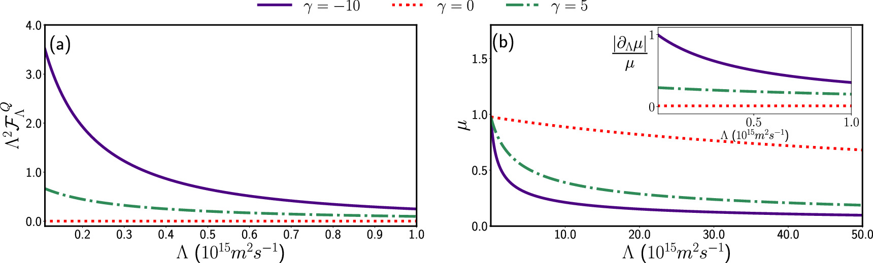
Figure 8. (a) QFI () and (b) purity μ as a function of environmental effect Λ for t = 50.0 μs, and considering the following values for the initial correlation: γ = − 10, γ = 0 and γ = 5. The inset in (b) shows the absolute relative variation , where we can see how it directly affects the way the QFI behaves. Also, note that initial correlated states with γ ≠ 0 show a more resilient QFI when compared with the standard uncorrelated Gaussian state, however, this does not necessarily result in a more robust purity.


Download figure:
Standard image High-resolution imageAppendix F.: Position-momentum correlations and Squeezing
Here we discuss the connection between PM correlation and squeezing for pure initial states. The correlated Gaussian state described by equation (1) was introduced in [28], where the real parameter γ ensures the correlation. The uncertainty in position and momentum for this initial state is given by and , whereas their covariance becomes


Exploring the correlation coefficient between and , i.e. , the γ parameter turns out to be , illustrating the physical meaning of γ as a parameter that encodes the initial correlations between and . Note that, it was explicitly considered the quantized operators and , with . Also, it was employed the symmetrization procedure to transform the product operator into a hermitian operator . From a practice point of view, this parameter can be seen as due to an atomic beam propagation along a transverse harmonic potential that effectively acts as a thin lens, which leads to a quadratic phase shift in the initial state [30] (see also appendix B). Furthermore, Gaussian correlated packets have been used in many contexts, for example in quantum optics [31].


![$[\hat{x},\hat{p}]=i\hslash $](https://content.cld.iop.org/journals/1402-4896/100/1/015111/revision2/psad9a18ieqn96.gif)


The variances in position and momentum for the dimensionless operators and are given by [34]


This shows that the correlated Gaussian state is not squeezed in terms of these conventional operators. On the other hand, in terms of the generalized quadratures and , which are defined in terms of and through a rotation in the phase space by an angle θ (; ), this state presents squeezing, as discussed in [34]. The variances of the new operators concerning the correlated Gaussian state are


For more details about the connection between PM correlations and squeezing we refer the reader to [35], where the variances of the operators and are investigated as a function of the rotation angle θ for the initially correlated Gaussian state.

