
Abstract
In this study, the fractional impacts of the beta derivative and M-truncated derivative are examined on the DNA Peyrard-Bishop dynamic model equation. To obtain solitary wave solutions for the model, the Sardar sub-equation approach is utilized. For a stronger comprehension of the model, the acquired solutions are graphically illustrated together with the fractional impacts of the beta and M-truncated derivatives. In addition to being simple and not needing any complicated computations, the approach has the benefit of getting accurate results.
Export citation and abstract BibTeX RIS

Original content from this work may be used under the terms of the Creative Commons Attribution 4.0 licence. Any further distribution of this work must maintain attribution to the author(s) and the title of the work, journal citation and DOI.
1. Introduction
Partial differential equations (PDEs) are very beneficial for the modeling and understanding of complicated processes in fields such as optics, fluid and solid mechanics, dynamical system propagation, chemical reactions in fluid dynamics, quantum theory, and others. Many researchers have thoroughly examined nonlinear partial differential equations (PDEs), and numerous techniques have been devised to address these PDEs. To obtain exact solutions to the nonlinear PDEs, various effective mathematical approaches have been utilized in the literature [1–14].
Recently, fractional calculus has gained a lot of attention from mathematicians as a new PDE study field. A differential equation with nonlinear terms and fractional derivatives incorporated is called a nonlinear fractional differential equation (NFDE). Integer-order derivatives are generalized into fractional derivatives. The ability of NFDEs to effectively simulate and assess a wide variety of real-world problems in fields including fluid mechanics, physics, biology, and more has drawn a lot of interest in recent years [15]. Various approaches and techniques have been developed to address NFDEs.
Fractional derivatives in physics have different meanings based on the situation they are used in. Fractional derivatives are used to simulate anomalous diffusion in systems where standard diffusion models are unable to sufficiently capture the spreading of particles, such as in porous media or complicated fluids. Fractional derivatives provide a mathematical tool to characterize the underlying dynamics in cases where the mean squared displacement of particles does not scale linearly with time, a phenomenon known as anomalous diffusion [16]. The behavior of viscoelastic materials, which have both elastic (spring-like) and viscous (fluid-like) qualities, is modeled using fractional derivatives. The non-local or memory effects in the material's reaction to stress or strain are captured by the fractional derivative [17]. Fractional derivatives are employed in fractal geometry and dynamics to characterize systems that display fractal behavior, including particle dispersion in fractal media or surface behavior. The dynamics of these systems in non-integer dimensions may be explained using a framework provided by fractional calculus [18]. Control theory is one area where fractional calculus has applications. Fractional derivatives are used to construct controllers for systems that include memory effects or non-local effects. For some kinds of dynamical systems, fractional controllers can offer better stability and performance [19]. In summary, fractional derivatives find applications in various physical phenomena involving non-local, memory-dependent, or anomalous behaviors. They provide a mathematical tool to describe complex systems more accurately than integer-order derivatives.
Soliton theory is very significant since many mathematical physics equations have soliton solutions. Solitons are solitary wave solutions that maintain their shape and amplitude while propagating through a medium. Analytical soliton solutions refer to exact mathematical expressions that describe these solitary waves in the context of differential equations. Soliton solutions are often found in various nonlinear partial differential equations (PDEs). When there are modifications to the phenomenon, such as disturbances, waves appear. When two or more solitons approach each other, an interaction occurs between them. Solitons are employed in optical fibers to transport digital information, which is the most significant technological utility. The soliton is a transverse electromagnetic wave that travels between two superconducting metal strips in electromagnets. As it turns out, one of the most attractive and interesting topics of research in many engineering and physical sciences has been these solutions. There is no doubt that solitary wave solutions contribute greatly to the interpretation of the physical properties of mathematical models. Recently, many researchers have addressed these solutions using various methods. A short list can be made as follows. The sub-equation method (see, [20–23]), the sine-cosine method (see, [24]), Laplace transform method (see, [25]), the auxiliary equation method (see, [26]), direct algebraic method (see, [27]), Kudryashov method (see, [28]), the variational iteration method (see, [29]), the first integral method (see, [30]), F-expansion method (see, [31, 32] ),  extension method (see, [33–35]), He's semi inverse method (see, [36]), ansatz approach (see, [37]) are some examples.
This paper is composed as follows: In section 2, the DNA Peyrard-Bishop model equation is mentioned and the equations to be solved are given. Since the equations to be solved involve Beta and M-truncated derivatives, their structure are briefly described in section 3. The recommended approach is explained in section 4. In section 5, a mathematical analysis of the model and its solutions by the suggested approach are presented. The effects of the fractional derivative on the solutions are given, and the results are shown for a few particular values in section 6. The results and the suitability of the approach are finally described in the final section.
2. The DNA Peyrard-Bishop dynamic model equation
Double helices are a common feature of DNA molecules. This implies that consists of two entangled, complementary polymeric chains [38]. B-shaped DNA is described by the Watson-Crick model as a double helix with two strings. It is reasonable to conclude that the crystal structure was homogenous since the masses of the nucleotides were not noticeably different. Since hydrogen bonds are employed to link strings, making them weak while keeping the harmonic longitudinal length strong, The PB model ignores all transverse displacements. The physical significance of the model lies in its ability to capture the essential features of DNA's structural dynamics, including the opening and closing of base pairs. This dynamic behavior is crucial for understanding processes like DNA replication, transcription, and repair, where the DNA molecule undergoes structural changes [39]. The equations in the literature and the Hamiltonian model of Peyrard and Bishop are both derived from Morse's potential as [39]

Here, the Morse potential is represented by the notation Uv (pk , rk ); pk, rk stand for the nucleotide displacements, and R, β for the depth and widht of the potential. Hamiltonian of the DNA chain was also described by [38]. In addition, Dauxois [40] presented an improved Peyrard-Bishop model. The Hamiltonian that explains hydrogen bonds cause strand apertures was given as [41–44].

where the strength of the linear and nonlinear couplings is shown by l1 and l2, respectively, wk = npk is the momentum for the displacement pk , and η is a constant. The equation of motion in the continuum limit may be expressed as follows, beginning with the Hamiltonian (2)

where  and d is the DNA ladder's intersite nucleotide distance [42–44]. As a consequence, the nonlinear evolution equation for the DNA Peyrard-Bishop dynamic model has been represented as

where c1, c2, A and Q = R are constants.
Using both the beta derivative and M-truncated derivative, the fractional order model associated with equation (4) is investigated in [45–49]. The DNA Peyrard-Bishop dynamic model in the following forms will be examined in this work.
It will be considered that the fractional DPB (DNA Peyrard-Bishop) model equation with the beta derivative is

where  is beta derivative introduced in section 3.1, and the M-truncated derivative is

where  is M-truncated derivative described in section 3.2.
3. The fundamental concepts of beta derivative and M-truncated derivative
3.1. The basic concepts of the beta derivative
Analytical solutions from NFDEs with beta derivatives are frequently beneficial in mathematical modeling. The fulfillment of the fractional chain rule by beta derivatives is a significant aspect of the analysis of fractional differential equations. Abdon Atangana [50–52] invented the term 'beta-derivative'. The suggested version's many components served as fractional derivative restraints and models for a variety of physical problems. They are a logical extension of the classical derivative, even though they are not fractional derivatives [53]. In contrast to well-known fractional derivatives, it has the following characteristics:
Suppose  . For 0 < μ ≤ 1 the beta derivative of ψ(λ) of order μ has been described in [50] as follows:

Some important properties of Beta Derivative are as follows:
-

-
, for any constant c,
-
-
-
,


where ψ and φ two functions μ differentiable and μ ∈ (0, 1].
Assuming that ψ is μ − differentiable on an open interval  , then
-
for all , then ψ is decreasing,
-
for all , then ψ is increasing,
-
for all , then ψ is constant.


These theorems and properties have been arised in [50–52].
Let  be given function. The beta fractional integral of ψ is defined by the following relation [51] :

3.2. The basic concepts of the M-truncated derivative
Pressume  and η > 0. For 0 < μ < 1, the truncated M-fractional derivative of v(η) of order μ has been defined by [54] as follows:

where  is a truncated single-parameter Mittag-Leffler function and defined as follows:

Functions h1(η) and h2(η), which are μ-derivable with 0 < ω ≤ 1 and δ > 0 at a point η > 0, satisfy the following properties [54, 55]:
-
, ,
-
,
-
,
-
, ,
- If h1 is differentiable, then ,
-
.


4. Brief description of Sardar subequation approach
The Sardar subequation approach, which was developed by Rezazadeh et al [56], is explained briefly in this section.
Let's consider an NLPDE in its general form

where F1 is a polynomial and the traveling wave equation as follows

where ν and γ are non-zero real constants. We may transform equation (11) into a nonlinear ordinary differential equation with the aid of equation (12):

where F2 is a polinomial in g( ) and the subscripts represent g()'s ordinary derivatives with regard to . We presume that equation (13) has the following solution:

where αi
s are real constants to be obtained (αN
≠ 0), N is a balancing number to be identified by utilizing the balancing rule to equation (13) and Φ() fulfills the following ordinary differential equation:

The solutions to equation (15) are as follows:
Case I. If k2 > 0 and k1 = 0, then
where
Case II. If k2 < 0, k3 > 0 and k1 = 0, then

where
Case III. If k2 < 0, k3 > 0 and  , then

where
Case IV. If k2 > 0, k3 > 0 and  , then

where
A set of algebraic equations for k2, k3, γ and αi
(i = 0, 1, 2,...,N) constants are obtained by substituting equation (14) into equation (13) , applying equation (15), adding all terms of the same degree of Φi
() and setting each coefficient of the resultant polynomial equal to zero. These values can be calculated with Maple and similar software programs. By substituting the determined constants and the known solutions of equation (15) into equation (14), the exact solutions of equation (11) are found.
5. Mathematical analysis of the model equation and its wave solutions
In this section, the approach briefly described above will be utilized for creating solitary wave solutions for the fractional DPB dynamic model equation. Let's consider equation (5) and equation (6). By applying the traveling wave transformation to these equations as follows,

for beta derivative:

for M-truncated derivative:

the following ordinary differential equation can be found as,

where γ is a constant. By multiplying the equation (19) by the value of  and applying integration on once, the following result is obtained

where K is a integration constant. For equation (20), by supposing the following

then, by adding equation (21) to equation (20), the nonlinear ordinary differential equation is constructed as follows:

If we take into the principle of homogeneous balance between the nonlinear variables f6 and the highest-order derivatives  or
or  in equation (22) , we have 4N + 4 = 6N, thus N = 2. Therefore, equation (14) takes the following form

It is substituted equation (23) and its derivatives into equation (22). After setting the coefficients of Φj (for j = 0, 1,...12) equal to zero, algebraic equations is formed. The following values of α0, α1, α2, γ, K, k1, k2 and k3 are gained by solving the nonlinear algebraic equations. Applying equation (23) to following solution sets and considering the cases of the method, the solitary wave solutions of the fractional DPB equation with respect to both derivatives are found.
Set 1.

Case I. If k2 > 0 and k1 = 0, then
Case II. If k2 < 0, k3 > 0 and k1 = 0, then
where for beta derivative
and for M-truncated derivative
Set 2.
Case III. If k2 < 0, k3 > 0 and  , then
Case IV. If k2 > 0, k3 > 0 and  , then

where for beta derivative

and for M-truncated derivative
6. Results and discussions
In this study, the solitary wave solutions of the fractional DPB dynamic model equation are obtained by using the well-known beta and M-truncated derivatives. The solutions are found while respecting the appropriate constraints, so as to avoid singularities and trivial solutions. Graphical illustrations of the physical behavior of the solutions achieved by the beta-derivatives and M-truncated derivatives are presented, along with their implementation in Maple. The fractional effects for this model with both derivatives are visually displayed on some of the solutions, given certain values for the free parameters. Each image shows fractional effects in both 3D and 2D for μ = 0.5. Figures 1 and 3 display the graphs for certain acceptable values of the hyperbolic solution, which were identified as p1(x, t) and p9(x, t), respectively. With the values A = − 1, Q = 0.01, c1 = 0.1, c2 = 0.01, ρ = ω = 1 (In figure 1, k2 = 1 and in figure 3, k2 = − 1), it demonstrated that the obtained solitary wave solutions display certain acceptable hyperbolic properties.

Figure 1. Graphical illustrations of p1(x, t).
Download figure:
Standard image High-resolution imagep3(x, t) and p12(x, t) have been exhibited in figures 2 and 4, respectively. When A = − 1, Q = 0.01, c1 = 0.1, c2 = 0.01, ρ = ω = 1 (In figure 2, k2 = − 1 and in figure 4, k2 = 1), the trigonometric solutions of the model in consideration are presented for μ = 0.5 value in these figures. By using both derivatives, the wave's shape seems to be consistent throughout the fractional order value, as the graphical representations clearly demonstrate.

Figure 2. Graphical illustrations of p3(x, t).
Download figure:
Standard image High-resolution image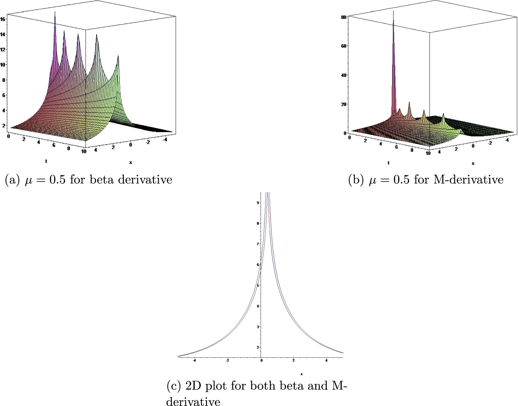
Figure 3. Graphical illustrations of p9(x, t).
Download figure:
Standard image High-resolution image
Figure 4. Graphical illustrations of p12(x, t).
Download figure:
Standard image High-resolution image
In all figures, for μ = 0.5, the 2D plots of the mentioned model at t = 1 are given. Moreover, the graphical representations make it clear that the application of both derivatives leads to a similar appearance of the wave shape.
7. Conclusion
In this study, the DPB dynamic model's solitary wave solutions are obtained. Two fractional derivatives, the beta derivative and the M-truncated derivative, have been effectively used to investigate the fractional effects of the suggested model. The suggested fractional model has been converted into an ordinary differential equation using a traveling wave transformation in conjunction with fractional operators. The Sardar sub-equation approach has been utilized to generate solitary wave solutions after getting the ordinary differential equation. Using both 2D and 3D plots, the dynamic behavior of the generated solutions has been examined by selecting particular values.
It is noteworthy that the suggested DPB dynamic model has been resolved using the Sardar sub-equation approach for the first time in order to extract solitary wave solutions. The suggested approach for obtaining hyperbolic and trigonometric solutions is incredibly dependable and efficient. The findings in this study, which are different from similar studies, can be very useful for describing the physical and dynamic properties of the biological population model, often referred to as the Peyrard-Bishop model. It is important to note that the applied approach is effective, adaptable, and strong for obtaining the solitons needed for usage in reality. The results acquired might be helpful for more research in engineering and physics.
Data availability statement
All data that support the findings of this study are included within the article (and any supplementary files).