
Abstract
For an undirected connected graph G = G(V, E) with vertex set V(G) and edge set E(G), a subset R of V is said to be a resolving in G, if each pair of vertices (say a and b; a ≠ b) in G satisfy the relation d(a, k) ≠ d(b, k), for at least one member k in R. The minimum set R with this resolving property is said to be a metric basis for G, and the cardinality of such set R, is referred to as the metric dimension of G, denoted by dimv(G). In this manuscript, we consider a complex molecular graph of one-heptagonal carbon nanocone (represented by HCNs) and investigate its metric basis as well as metric dimension. We prove that just three specifically chosen vertices are enough to resolve the molecular graph of HCNs. Moreover, several theoretical as well as applicative properties including comparison have also been incorporated.
Export citation and abstract BibTeX RIS

Original content from this work may be used under the terms of the Creative Commons Attribution 4.0 licence. Any further distribution of this work must maintain attribution to the author(s) and the title of the work, journal citation and DOI.
1. Introduction
The molecular structure of a compound is frequently illustrated by a graph in chemical graph theory (CGT), where the atoms and bonds present in the chemical compound are respectively represented by vertices and edges [1]. In CGT, several restrictions were made on a molecular structure, for instance, multiple bonds (edges) between the atoms can be considered as a single bond (edge) (i.e., no multiple edges between any two vertices are considered) and the hydrogen atoms are not considered here due to their unique valency (i.e., the valency of the hydrogen atom is 1). Therefore, we simply remove the vertices corresponding to the hydrogen atom. As a result of these restrictions, the structure of a compound can be referred to as a molecular graph in CGT [2]. In order to understand the concept, we consider an example below, in which the figure 1(A) is the chemical structure, and figure 1(B) is its corresponding molecular graph. The majority of the chemical compounds under study are carbon-based compounds, with vertex (atom) degrees not more than 4. It is also important to note that, some authors, refer to the term molecular graph as chemical graphs, in which the vertex degrees are bounded above by 4 [3].
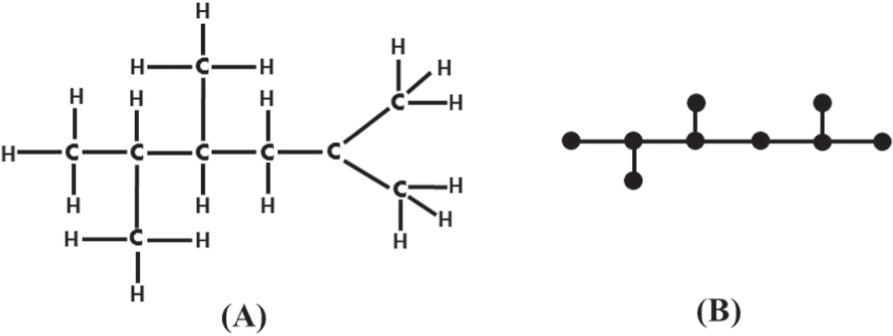
Figure 1. (A) Chemical Structure of C9 H20 and (B) Molecular Graph of C9 H20.
Download figure:
Standard image High-resolution imageThe theoretical aspects pertaining to molecular graphs is a subject of graph theory, specifically CGT, that deals with both mathematics and chemistry. The fundamental role of CGT is to get a deeper insight into a molecular structure, that are enormous and complicated in their natural forms Then, for these complex chemical structures, the valuable contribution of CGT is to understand these structures and extract massive theoretical and applicative knowledge corresponding to its molecular graph [4]. In short, CGT helps us to make it possible to capture the fundamental characteristics of the complex chemical structure of a chemical compound. This can be done by investigating several topological descriptors/indices or by assigning certain distinct as well as unique distance codes for each member (atoms or/and bonds) present in a chemical compound's molecular structure [5–7]. The notion with which one defines the unique position of each member of a graph with respect to some selected set of vertices (landmark vertices) is known as the metric dimension [6, 7]. In this manuscript, we consider a family of molecular graphs known as carbon nanocones (particularly, one-heptagonal carbon nanocones (HCN)) and investigate its metric basis set as well as the metric dimension. In the next portion, a concise overview of the carbon nanocone as well as HCN will be presented, followed by an exploration of its diverse range of applications.
Carbon nanocones (CNCs) which belong to the class of carbon nanomaterials, were first identified by Sattler and Ge [8]. These conical formations are made primarily of carbon and have at least one dimension of the order of one micrometer or less. CNCs have the same height as their diameter, as contrasted with nanowires with tips, which are much longer than their diameter. CNCs occur on the surface of naturally occurring graphite. These CNCs are made by cutting a wedge of graphene at an angle of 60 degrees, joining the edges, and producing a cone with a single flaw at the tip (flaw is k-sided, where k is odd natural, with k ≥ 5). One more method is that, when hydrocarbons are broken down with the help of a plasma torch, CNCs are produced. The opening angle (apex) of cones has optimal values of approximately 60, 40, and 20 degrees from the perspective of electron microscopy. Negative curvature, as shown in figure 2, is completely due to the addition of heptagons to the hexagonal lattice. Furthermore, the existence of the single sevenfold in the ordinary graphene lattice has only been studied theoretically, it is known as the one-heptagonal carbon nanocone, denoted by HCNs , and this situation has not yet been verified experimentally, it has been proposed that it may exist [9].
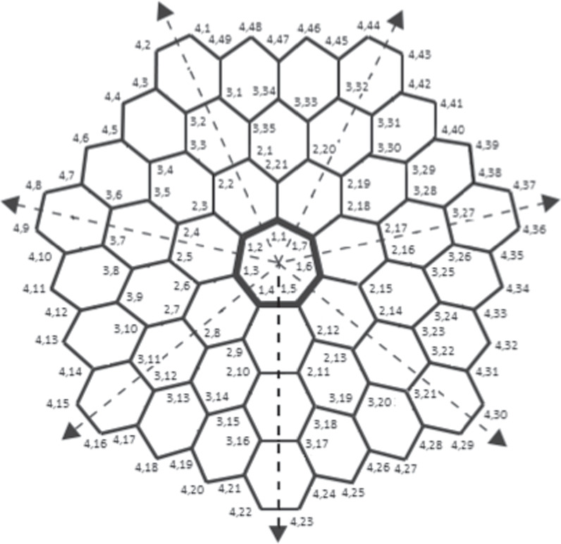
Figure 2. Generalized Molecular Graph of HCNs .
Download figure:
Standard image High-resolution imageSeveral papers regarding the chemical structure of HCNs
have been reported in the last two decades. For instance, to obtain the Wiener index of HCNs
whenever 1 ≤ s ≤ 15, a polynomial is given by employing a Java program and the curve fitting method [10]. The polynomial by which one can get the Wiener index for HCNs
with 1 ≤ s ≤ 15 is given by:  , where f, e, d, c, b, and a are some numerical fixed values. Next, for all s in HCNs
, Ashrafi and Mohammad-Abadi [11] determine the Wiener index by utilizing Sandi Klavzar's algorithm [12]. The final formula to obtain the Wiener index is thus given as follows:
, where f, e, d, c, b, and a are some numerical fixed values. Next, for all s in HCNs
, Ashrafi and Mohammad-Abadi [11] determine the Wiener index by utilizing Sandi Klavzar's algorithm [12]. The final formula to obtain the Wiener index is thus given as follows:  . Moreover, a polynomial, known as the Hosaya polynomial, was investigated by Xu and Zhang [13] and a certain number of generalizations were made on various distinct results already available for HCNs
[11].
. Moreover, a polynomial, known as the Hosaya polynomial, was investigated by Xu and Zhang [13] and a certain number of generalizations were made on various distinct results already available for HCNs
[11].
Because of their durability and adaptability, CNCs are well-suited for manipulating other nanoscale structures, hinting that they will play an important role in engineering nanotechnology. The applications of 3D carbon structures, i.e., CNCs were reported in many disciplines, which include field emission transistors, power storage devices, high-performance catalysis, implants & other biomedical technology, photovoltaics, supercapacitors, etc [14]. Therefore, we are highly motivated as well as interested in contributing more to this topic due to its wide-ranging applications, uses, and significance across numerous academic disciplines.
In physics, CNCs exhibit unique electronic properties owing to their distinct geometric structures, such as pentagonal and heptagonal defects, which enable exploration into novel material science applications, including site-specific functionalization via free radicals, as demonstrated in computational studies [15]. Additionally, CNCs have shown promising characteristics as thermal rectifiers, where molecular dynamic simulations revealed pronounced thermal rectification over a wide temperature range, highlighting their potential significance in thermoelectric and energy conversion systems. So, this shows that the CNCs have relevant applicability in both electronic and thermal aspects of physics, contributing to advancements in energy technology and material science [16, 17]. Carbon atoms in HCNs and the connections between them serve as vertices and edges in HCNs , respectively. Since no results exist regarding the metric basis and dimension of HCNs . Therefore, we investigate these graph parameters as well as certain fundamental properties of this complex molecular graph of HCNs in this paper.
For a simple, connected, and undirected graph G = (V, E), the idea of metric dimension is just comparable to the number of satellites (in total) required for the perfect operation of GPS (Global Positioning Systems). The key concept behind metric dimension, is that a small ordered set, say U, is selected from the vertex set V(G), and the members of U are called as satellites or landmarks [18, 19]. Then, using the distance of all vertices from the landmarks, one can uniquely identify each vertex in V(G) corresponding to the set U. The solution to such a problem for several complex graph structures is hard to get, but significant information can be provided by it, in order to tackle many complicated situations [7]. For instance, the small set U can assist robots navigating in a physical space, identifying intersection points on roads, uniquely specifying a group of people by assigning a UIN (unique identification number), or tracing disease transmission between distinct regions [9, 20]. This might be employed as well for more general activities like recognizing a source of lies and deceitful information in a network of people, comparing distinct architectures of networks, chemical structure categorization, or quantitatively encoding symbolic data [19].
Slater [7] was the first to introduce the concept of metric dimension and resolving set (under the name locating numbers and locating set resp.), and later Harary & Melter [6] also studied the same concept. But the idea of dimension of a graph was already presented by Erdos et al [21], in which they have proposed a natural geometrical description of a graph's dimension and also to investigate some of its ramifications. Talking about the two initial papers [6, 7], the authors mainly focus on the tree graph's metric dimension and simply provide the exact formulas for the same. They have briefly discussed the metric dimension of numerous varieties of graphs, including cycle graphs, complete graphs, and bipartite graphs (complete), but incorrectly report the metric dimension of wheel graphs as two in the same paper [6]. By utilizing the fact, that the distance between the resolving set elements and all the vertices in G, they have proposed an algorithm in order to reconstruct the tree graph for which the resolving set has been drawn. Although this is not possible for all generic graphs because not every edge is guaranteed to be represented by the shortest possible path, with the end vertex as a member of the taken resolving set.
After the introduction of these notions, several authors reported the advancement of these concepts, which includes, their theoretical aspects, application, and many distinct variants. These concepts have a countable set consisting of a wide range of applications in various scientific disciplines, for instance, the unique determination of intersection points on the roads [9], pattern recognition and image processing [22], robot navigation [23], verification and network discovery [24], connected joins and graph-theoretic medicinal chemistry [18], mastermind games involving several strategies [25], etc. The reported studies regarding the investigation of metric dimensions for various significant families, like one-pentagonal carbon nanocone, heptagonal circular ladder, mobious ladder, and many chemical graphs, refer to [26–29]. The problem in deciding to or not to obtain  , for any connected graph G and a positive integer h, is still computationally intractable, which is also known as an NP-complete problem [30, 31].
The computation of metric dimension for molecular graph families is always a challenging task because deciding/selecting landmark vertices (atoms) in minimum numbers is not that easy due to the complexity and scalability of the structures [30]. Although, several authors studied metric dimension and its related variants for several distinct complex molecular graphs as well as for various other graph-theoretic aspects, for example, the metric dimension of H-Napthalenic nanotubes as well as VC5 C7 were investigated in [32]; edge metric basis and the dimension of one-pentagonal and one-heptagonal carbon nanocone was investigated [9, 20] respectively; for cellulose networks an estimated upper bounds were provided for the cardinality of their resolving sets [33]; the metric dimension of Alpha & 2D lattice boron nanotubes were reported [34]; for polycyclic aromatic hydrocarbons several variants of metric dimension were investigated [35, 36]; for chemical graphs of starphene and hollow coronoid several metric dimension variants were reported [37–39]. For certain chemical as well as planar graphs, these variants are investigated [20, 27, 28].
The notion of metric dimension was extended and investigated by eminent researchers from time to time, who named them variants of metric dimension [9]. These variants of metric dimension have been studied from both an applicative and theoretical perspective. They have investigated these notions for several significant families of graphs, for instance, path graphs, complete graphs, cycle graphs, cycle graphs with chords, antiprism graphs, several ladder graphs (pentagonal, heptagonal, etc.), convex polytope graphs, wheel graphs, tadpole graphs, kayak paddle graphs, and numerous planar and chemical graphs [27, 32, 33, 37, 38, 40]. Even after investigating these notions for the large number of graph families, there are still many families for which these notions have not been investigated to date. So, in this manuscript, we consider an interesting graph family of chemical compounds known as one-heptagonal carbon nanocones, denoted by HCNs , and determine its metric basis as well as metric dimension. In view of the wide range of applicability of carbon nanocones, as discussed above, it is also a need to contribute more on this subject.
The structure of the manuscript is systematized in the following manner: section 2 emphasizes the basic definitions in graph theory, in particular resolving sets, metric basis, and metric dimension; section 3 contributes towards the major findings, including a comparison of the aforementioned parameters for the family of a complex graph of HCNs ; section 4 emphasizes some extra properties (like independence) pertaining to the minimum resolving set for HCNs ; and finally, all the outcomes, including future scope related to our study, are reported in the conclusion.
2. Preliminaries
Throughout this article, all graphs taken into consideration are planar, connected, non-trivial, undirected, and simple. In order to carry out the basics of graph theory, we are following these books [41, 42]. Consider a graph, denoted by G = (V, E), where V(G) and E(G) are referred to be its vertex and edge sets respectively. The cardinality of the vertex and edge sets, i.e., ∣V(G)∣ and ∣E(G)∣, represents the order and size of G respectively. The totality of distinct edges in the shortest length path between two different vertices k1 and k2 in V(G), is referred to as the distance between k1 and k2 in G, denoted by d(k1, k2). The number of distinct edges touching a vertex k in G is called the degree (valency) of a vertex k, denoted by dk . Further, a graph is referred to as a regular graph if the degree of every vertex within the graph is identical.
Two vertices k1 and k2 in a connected graph G are said to be resolved by a vertex k, if d(k, k1) ≠ d(k, k2) in G. Then, a subset U ⫅ V(G) with this property, i.e., every pair of different vertices in G can be resolved by at least one member of U, is said to be a resolving set (RS) for G. The smallest cardinality set U with a resolving characteristic is called the metric basis (MB) for G, and the MB set cardinality is the metric dimension (MD) for G, represented by dimv (G) [6, 7].
For a subset U = {k1, k2, k3,...,ks } of distinct ordered vertices in V(G), the unique s-length tuple code for each k ∈ V(G) is given as follows: cv (k∣U) = (d(k, k1), d(k, k2), d(k, k3),...,d(k, ks )) (also known as metric code/vertex code/metric representation). Using this fact, the subset U is a RS for G, if cv (k1∣U) ≠ cv (k2∣U), for every pair of different vertices k1, k2 ∈ V(G). To show that a subset U in V(G) is resolving in G, it is sufficient to show that cv (k1∣U) ≠ cv (k2∣U), for all k1, k2 ∈ V(G)\U. Next, a subset U in V(G) with distinct vertices is said to be a resolving independent set (RIS) for G, if it is (i) an independent set as well as (ii) a RS in G. A proper subset of a RS is not necessarily a RS, while a superset of every RS is always a RS in G [43].
For several significant graphs, for instance, the path graph, complete graph, and cycle graph of order m and size k are denoted by Pm , Km , and Cm respectively. The MD for these basic graphs is given as follows:
Proposition 1. [20]  ,
,  , and
, and  for every
  .
.
From this proposition, we clearly observe that, for any m vertex graph G and a positive integer g, we find that 1 ≤ g ≤ m − 1; where  .
.
Example 2.1. To understand the concept of RS and MD, let us consider a graph G1 of order 16 and size 22 (see figure 3). We suppose that a set U with cardinality 2, is RS for G1. Since the graph G1 has 16-vertices and the set U consists of two vertices, the possible number of combinations for set U with two vertices is equal to  . Next, on arbitrary, we suppose that
  . Then, by definition of MD, we have
  , a contradiction. Based on the complexity and symmetry of the graph G1, during the analysis, similar contradictions were found in the remaining 119 cases. Thus, the set U with two vertices can never be a RS for G1, i.e.,
  . But the set
  is a resolving set for G1. This can be seen in the table 1 below, as all the vertex codes for 16-vertices in G1 are unique, corresponding to the set U1. Hence, the set U1 is the MB for the graph G1 and this implies that
  .
.

Figure 3. Graph G1.
Download figure:
Standard image High-resolution imageTable 1. Vertex codes for 16-vertices in G1 with respect to the set U1 = {p1, p4, p13}.
| Vertices pi | Metric codes | Vertices pi | Metric codes |
|---|---|---|---|
| p1 | (0, 3, 3) | p9 | (2, 4, 1) |
| p2 | (1, 2, 4) | p10 | (3, 3, 2) |
| p3 | (2, 1, 4) | p11 | (3, 3, 3) |
| p4 | (3, 0, 5) | p12 | (4, 2, 4) |
| p5 | (1, 4, 2) | p13 | (3, 5, 0) |
| p6 | (2, 3, 3) | p14 | (4, 4, 1) |
| p7 | (3, 2, 3) | p15 | (4, 4, 2) |
| p8 | (4, 1, 4) | p16 | (5, 3, 3) |
One-Heptagonal Carbon Nanocone: We consider a family of a molecular graph known as one-heptagonal carbon nanocone, and we represent this family by the symbol HCNs
(where s ≥ 2) throughout this manuscript and it shown in figure 4. It is different from the hexagonal honeycomb layer as it consists of a single 7 vertex/edge cycle lying at its core (middle), and this core cycle is surrounded by the layers of hexagonal rings in a manner that; the first layer consists of 7 hexagonal rings, the second layer consists of 14 hexagonal rings, the third layer consists of 21 hexagonal rings, and so on, the sth
layer consists of 7s hexagonal rings. The total number of distinct faces in HCNs
are  ; in which HCNs
has
; in which HCNs
has  hexagonal faces, 1 seven sided cycle, and an outer face. The graph HCNs
has in total
hexagonal faces, 1 seven sided cycle, and an outer face. The graph HCNs
has in total  number of edges and 7s2 number of vertices. It is important to note that the graph of HCNs
has vertices of degrees two and three only, if we observe it closely, we find that the vertices of degree two are lie on the outermost cycle in HCNs
. For our convenience, we denote the set of vertices in HCNs
by
number of edges and 7s2 number of vertices. It is important to note that the graph of HCNs
has vertices of degrees two and three only, if we observe it closely, we find that the vertices of degree two are lie on the outermost cycle in HCNs
. For our convenience, we denote the set of vertices in HCNs
by  and the set of edges in HCNs
by
and the set of edges in HCNs
by  . These sets, i.e.,
  &
&  in HCNs
are presented as follows:
in HCNs
are presented as follows:

Figure 4. General Graph of HCNs .
Download figure:
Standard image High-resolution image
 and
and

{q1,1 q2,21, q1,2 q2,3, q1,3 q2,6, q1,4 q2,9, q1,5 q2,12, q1,6 q2,15, q1,7 q2,18} ∪
{qb,1 qb+1,14(b+1)−7, qb,2l qb+1,2l+1∣ 1 ≤ l ≤ b; 2 ≤ b ≤ s − 1} ∪
{qb,2l−1 qb+1,2l+2∣b + 1 ≤ l ≤ 2b; 2 ≤ b ≤ s − 1} ∪ {qb,2l−2 qb+1,2l+3∣2b + 1 ≤ l ≤ 3b; 2 ≤ b ≤ s − 1} ∪
{qb,2l−3 qb+1,2l+4∣3b + 1 ≤ l ≤ 4b; 2 ≤ b ≤ s − 1} ∪ {qb,2l−4 qb+1,2l+5∣4b + 1 ≤ l ≤ 5b; 2 ≤ b ≤ s − 1} ∪
{qb,2l−5 qb+1,2l+6∣5b + 1 ≤ l ≤ 6b; 2 ≤ b ≤ s − 1} ∪
{qb,2l−6 qb+1,2l+7∣6b + 1 ≤ l ≤ 7b − 1; 2 ≤ b ≤ s − 1}.
The edge metric basis and edge metric dimension, denoted by dime (G), for the graph of HCNs have been investigated by Sharma et al [9], and regarding this variant of MD, they proved the following result:


Next, it is interesting to note that the MD and MB for the graph of HCNs have not been reported to date. So, in this paper, we consider the almost 3-regular graph of HCNs and examine its RS, basis set, as well as MD. In this graph, it is very important to select the vertices for their minimum RS. Therefore, in order to cover this research gap, we will select appropriate resolving vertices and finally, investigate its MB, including its MD.
3. Methodology
To elucidate our main results, the methodology employed in our research is as follows:
All the results obtained in the manuscript are theoretical, so in order to prove them, we simply employ an abstract-theoretical and philosophical approach. In particular, the scientific method approach has been adopted in order to carry out the proof of the results.
Procedure: The selection of resolving vertices in HCNs is entirely based on the graph vertices, edges, symmetry, shape, and size (verification is done manually for the larger number of hexagonal layers). Next, for bounded and constant MD, two approaches were made, (i) we will give representation to every vertex of the graph, in order to get the upper bound for the above mentioned notion, and (ii) for lower bounds, we will either use the existing results or obtain contradictions.
4. Minimum resolving number for HCNs
Chemical parameters/indices is one of the most fundamental concepts that is increasingly employed in chemical graph theory nowadays. The purpose is to correlate a numerical value with a graph structure, which frequently has some form of correlation with the properties of associated compounds. For this reason, these significant chemical indices are commonly used as descriptors of chemical structures. A graph-theoretical study of such a chemical parameter often entails analyzing its behavior in various types of graphs, including upper and lower bounds as well as minima and maxima in terms of various graph characteristics. In the same direction, resolvability parameters are a recently introduced concept in which an entire molecular structure is designed in such a manner that every element (bonds or atoms) gets its position uniquely. In particular, we investigate the minimum RS as well as MD for HCNs in this section.
Theorem 2. For every  , we have
  .
.
Proof. This can be proved easily by constructing a RS (say, Hs
) in such a way that its cardinality is less than or equal to three and the vertices are selected in such a manner that every vertex present in HCNs
has unique identification with respect to that particular chosen RS. For this, suppose  , where these three vertices are chosen in a very precise manner (for the position of these three selected vertices, refer to figure 4 and the vertices in red color).
Claim: Hs with three vertices is a RS for HCNs .
To show this, we employed a technique by which we assign metric representations to each member present in  corresponding to the set Hs
. We further show that all the representations are unique in
corresponding to the set Hs
. We further show that all the representations are unique in  with respect to Hs
.
with respect to Hs
.
Metric representations in HCNs for the first two inner cycles are listed in table 2 below:
Metric representations in HCNs for the third cycle from inner side are listed in table 3 below:
We use the symbols E and O instead for even and odd numbers. After third cycle, the metric representation for vertices of bth
 ) cycle are listed below in table 4:
Lastly, for the outermost cycle vertices in HCNs
, i.e.,  cycle, the vertex representations are listed below in table 5:
The vertex representations for all the vertices present in HCNs
are listed in the four tables 2- 5 above. We notice that for all the members present in  , the metric representations are distinct as well as unique, i.e.,
  for any pair of v1 and v2 present in
  . Therefore, on the basis of these observations, we are able to conclude that the set Hs
with three vertices is a RS for a complex graph of HCNs
and thus, we have
. Therefore, on the basis of these observations, we are able to conclude that the set Hs
with three vertices is a RS for a complex graph of HCNs
and thus, we have  .□
.□
Table 2. HCNs with vertex representations for vertices of its inner two cycles.
| Vertices | Codes | Vertices | Codes |
|---|---|---|---|
| q1,1 | (2s − 2, 2s − 2, 2s + 1) | q1,2 | (2s − 1, 2s − 3, 2s) |
| q1,3 | (2s, 2s − 2, 2s − 1) | q1,4 | (2s + 1, 2s − 1, 2s − 2) |
| q1,5 | (2s + 1, 2s, 2s − 1) | q1,6 | (2s, 2s, 2s) |
| q1,7 | (2s − 1, 2s − 1, 2s + 1) | q2,1 | (2s − 4, 2s − 4, 2s + 3) |
| q2,2 | (2s − 3, 2s − 5, 2s + 2) | q2,3 | (2s − 2, 2s − 4, 2s + 1) |
| q2,4 | (2s − 1, 2s − 3, 2s + 2) | q2,5 | (2s, 2s − 2, 2s + 1) |
| q2,6 | (2s + 1, 2s − 1, 2s) | q2,7 | (2s + 2, 2s, 2s − 1) |
| q2,8 | (2s + 3, 2s + 1, 2s − 2) | q2,9 | (2s + 2, 2s, 2s − 3) |
| q2,10 | (2s + 3, 2s + 1, 2s − 4) | q2,11 | (2s + 3, 2s + 2, 2s − 3) |
| q2,12 | (2s + 2, 2s + 1, 2s − 2) | q2,13 | (2s + 3, 2s + 2, 2s − 1) |
| q2,14 | (2s + 2, 2s + 2, 2s) | q2,15 | (2s + 1, 2s + 1, 2s + 1) |
| q2,16 | (2s + 2, 2s + 2, 2s + 2) | q2,17 | (2s + 1, 2s + 1, 2s + 3) |
| q2,18 | (2s, 2s, 2s + 2) | q2,19 | (2s − 1, 2s − 1, 2s + 3) |
| q2,20 | (2s − 2, 2s − 2, 2s + 3) | q2,21 | (2s − 3, 2s − 3, 2s + 2) |
Table 3. HCNs with vertex representations for vertices of its third cycle.
| Vertices | Codes | Vertices | Codes |
|---|---|---|---|
| q3,1 | (2s − 6, 2s − 6, 2s + 5) | q3,2 | (2s − 5, 2s − 7, 2s + 4) |
| q3,3 | (2s − 4, 2s − 6, 2s + 3) | q3,4 | (2s − 3, 2s − 5, 2s + 4) |
| q3,5 | (2s − 2, 2s − 4, 2s + 3) | q3,6 | (2s − 1, 2s − 3, 2s + 4) |
| q3,7 | (2s, 2s − 2, 2s + 3) | q3,8 | (2s + 1, 2s − 1, 2s + 2) |
| q3,9 | (2s + 2, 2s, 2s + 1) | q3,10 | (2s + 3, 2s + 1, 2s) |
| q3,11 | (2s + 4, 2s + 2, 2s − 1) | q3,12 | (2s + 5, 2s + 3, 2s − 2) |
| q3,13 | (2s + 4, 2s + 2, 2s − 3) | q3,14 | (2s + 5, 2s + 3, 2s − 4) |
| q3,15 | (2s + 4, 2s + 2, 2s − 5) | q3,16 | (2s + 5, 2s + 3, 2s − 6) |
| q3,17 | (2s + 5, 2s + 4, 2s − 5) | q3,18 | (2s + 4, 2s + 3, 2s − 4) |
| q3,19 | (2s + 5, 2s + 4, 2s − 3) | q3,20 | (2s + 4, 2s + 3, 2s − 2) |
| q3,21 | (2s + 5, 2s + 4, 2s − 1) | q3,22 | (2s + 4, 2s + 3, 2s) |
| q3,23 | (2s + 3, 2s + 3, 2s + 1) | q3,24 | (2s + 4, 2s + 4, 2s + 2) |
| q3,25 | (2s + 3, 2s + 3, 2s + 3) | q3,26 | (2s + 4, 2s + 4, 2s + 4) |
| q3,27 | (2s + 3, 2s + 3, 2s + 5) | q3,28 | (2s + 2, 2s + 2, 2s + 4) |
| q3,29 | (2s + 1, 2s + 1, 2s + 5) | q3,30 | (2s, 2s, 2s + 4) |
| q3,31 | (2s − 1, 2s − 1, 2s + 5) | q3,32 | (2s − 2, 2s − 2, 2s + 5) |
| q3,33 | (2s − 3, 2s − 3, 2s + 4) | q3,34 | (2s − 4, 2s − 4, 2s + 5) |
| q3,35 | (2s − 5, 2s − 5, 2s + 4) |
Table 4. HCNs with vertex representations for vertices of its bth (4 ≤ b ≤ s − 1) cycle.
| Vertices | Codes |
|---|---|
| qb,l ; l = 1 | (2s − 2b, 2s − 2b, 2s + 2b − 1) |
| qb,l ; 2 ≤ l(E) ≤ 2b | (2s − 2b + l − 1, 2s − 2b + l − 3, 2s + 2b − 2) |
| qb,l ; 2 ≤ l(O) ≤ 2b | (2s − 2b + l − 1, 2s − 2b + l − 3, 2s + 2b − 3) |
| qb,l ; 2b + 1 ≤ l ≤ 4b | (2s − 2b + l − 1, 2s − 2b + l − 3, 2s + 2b − l + 6) |
| qb,l ; 4b + 1 ≤ l(E) ≤ 6b − 2 | (2s + 2b − 1, 2s + 2b − 3, 2s + 2b − l + 6) |
| qb,l ; 4b + 1 ≤ l(O) ≤ 6b − 2 | (2s + 2b − 2, 2s + 2b − 4, 2s + 2b − l + 6) |
| qb,l ; 6b − 1 ≤ l(E) ≤ 8b − 2 | (2s + 2b − 2, 2s + 2b − 3, 2s − 8b + l + 2) |
| qb,l ; 6b − 1 ≤ l(O) ≤ 8b − 2 | (2s + 2b − 1, 2s + 2b − 2, 2s − 8b + l + 2) |
| qb,l ; 8b − 1 ≤ l(E) ≤ 10b − 3 | (2s + 2b − 2, 2s + 2b − 2, 2s − 8b + l + 2) |
| qb,l ; 8b − 1 ≤ l(O) ≤ 10b − 3 | (2s + 2b − 3, 2s + 2b − 3, 2s − 8b + l + 2) |
| qb,l ; 10b − 2 ≤ l(E) ≤ 12b − 5 | (2s + 12b − l − 6, 2s + 12b − l − 6, 2s + 2b − 2) |
| qb,l ; 10b − 2 ≤ l(O) ≤ 12b − 5 | (2s + 12b − l − 6, 2s + 12b − l − 6, 2s + 2b − 1) |
| qb,l ; 12b − 4 ≤ l(E) ≤ 14b − 7 | (2s + 12b − l − 6, 2s + 12b − l − 6, 2s + 2b − 1) |
| qb,l ; 12b − 4 ≤ l(O) ≤ 14b − 7 | (2s + 12b − l − 6, 2s + 12b − l − 6, 2s + 2b − 2) |
Table 5. HCNs with vertex representations for vertices of its b = sth cycle.
| Vertices | Codes |
|---|---|
| qs,l ; l = 1 | (0, 2, 4s − 1) |
| qs,l ; l = 2 | (1, 1, 4s − 2) |
| qs,l ; 3 ≤ l(E) ≤ 2b | (l − 1, l − 3, 4s − 2) |
| qs,l ; 3 ≤ l(O) ≤ 2b | (l − 1, l − 3, 4s − 3) |
| qs,l ; 2b + 1 ≤ l ≤ 4b | (l − 1, l − 3, 4s − l + 8) |
| qs,l ; 4b + 1 ≤ l(E) ≤ 6b − 2 | (4s − 1, 4s − 3, 4s − l + 8) |
| qs,l ; 4b + 1 ≤ l(O) ≤ 6b − 2 | (4s − 2, 4s − 4, 4s − l + 8) |
| qs,l ; 6b − 1 ≤ l(E) ≤ 8b − 2 | (4s − 2, 4s − 3, l − 6s + 2) |
| qs,l ; 6b − 1 ≤ l(O) ≤ 8b − 2 | (4s − 1, 4s − 2, l − 6s + 2) |
| qs,l ; 8b − 1 ≤ l(E) ≤ 10b − 3 | (4s − 2, 4s − 2, l − 6s + 2) |
| qs,l ; 8b − 1 ≤ l(O) ≤ 10b − 3 | (4s − 3, 4s − 3, l − 6s + l + 2) |
| qs,l ; 10b − 2 ≤ l(E) ≤ 12b − 6 | (14s − l − 6, 14s − l − 6, 4s − 2) |
| qs,l ; 10b − 2 ≤ l(O) ≤ 12b − 6 | (14s − l − 6, 14s − l − 6, 4s − 1) |
| qs,l ; l = 12b − 5 | (14s − l − 6, 14s − l − 4, 4s − 1) |
| qs,l ; 12b − 4 ≤ l(E) ≤ 14b − 7 | (14s − l − 6, 14s − l − 4, 4s − 1) |
| qs,l ; 12b − 4 ≤ l(O) ≤ 14b − 7 | (14s − l − 6, 14s − l − 4, 4s − 2) |
Next, to complete the proof, we have to investigate the reverse inequality for the MD of HCNs
, i.e.,  . This can be done by simply showing that for HCNs
, no set Hs
with less than or equal to two vertices (i.e., ∣Hs
∣ ≤ 2) form a RS for HCNs
.
. This can be done by simply showing that for HCNs
, no set Hs
with less than or equal to two vertices (i.e., ∣Hs
∣ ≤ 2) form a RS for HCNs
.
Theorem 3. For every  , we have
  .
.
Proof. This inequality for HCNs
can be easily achieved, if we simply prove that, no set Hs
in HCNs
having  , is able to resolve all the vertices present in HCNs
. First, we assume that
, is able to resolve all the vertices present in HCNs
. First, we assume that  , and it is proved that
  if and only if
  , where Ps
is a path graph of order s, so for the complex graph of HCNs
, a set Hs
with
, where Ps
is a path graph of order s, so for the complex graph of HCNs
, a set Hs
with  can never be a RS [27]. Next, we were only left with the case, when
  . Then, we select two vertices from
  for Hs
, on an arbitrary basis and prove that the set Hs
can never be a RS in HCNs
. In order to get this, we suppose, on the contrary, that Hs
with cardinality 2, completely resolves all the members in
for Hs
, on an arbitrary basis and prove that the set Hs
can never be a RS in HCNs
. In order to get this, we suppose, on the contrary, that Hs
with cardinality 2, completely resolves all the members in  . Suppose
  . Then, depending upon the selection of the vertices in Hs
, we have to discuss the following three possibilities:
. Then, depending upon the selection of the vertices in Hs
, we have to discuss the following three possibilities:
Case 1. When the two vertices  and
and  in Hs
are from the same mth
-cycle, i.e.,
in Hs
are from the same mth
-cycle, i.e.,  . Then
  .
.
Table 6 and figure 5 shows that the contradictions can be verified easily for subcases 1 and 3. But for subcase second, when  , we found that the end vertex on the bth
cycle i.e.,
, we found that the end vertex on the bth
cycle i.e.,  colored in black and the other vertices on bth
cycle, which are colored in yellow, red, purple, and green, are at equal distance, from the pair of vertices in the set A1, A2, A3, and A4 respectively (where
colored in black and the other vertices on bth
cycle, which are colored in yellow, red, purple, and green, are at equal distance, from the pair of vertices in the set A1, A2, A3, and A4 respectively (where  ,
,  ,
,  , and
, and  ), which is a contradiction.
Case 2. When the two vertices  and
and  in Hs
are from two distinct cycles, i.e.,
in Hs
are from two distinct cycles, i.e.,  lies on
  cycle and
  lies on
  cycle.
Table 7 and figure 6 shows that the contradiction can be verified easily for subcase 1. But for subcase second, when  , we found that the first vertex on the bth
cycle i.e.,
, we found that the first vertex on the bth
cycle i.e.,  and the vertices on
  cycle, which is colored in yellow, red, purple, and green, are at an equal distance, from the pair of vertices in the set A1, A2, A3, and A4 respectively (where
  ,
,  ,
,  , and
, and  ), which is a contradiction.
Case 3. When the two vertices  and
and  in Hs
are from two distinct non-adjacent cycles i.e.,
in Hs
are from two distinct non-adjacent cycles i.e.,  lies on mth
cycle and
lies on mth
cycle and  lies on nth
cycle, where the difference between m and n is
lies on nth
cycle, where the difference between m and n is  i.e.,
i.e.,  . For this case, refer to table 8 and figure 7 below.
In the first subcase, we find that the first vertex on the first cycle, i.e.,  and the vertices on bth
(
and the vertices on bth
( ) cycle, which is colored in red, yellow, purple, and green are at an equal distances, from the pair of vertices in the set A1, A2, A3, and A4 respectively (where
  ,
,  ,
,  , and
, and  ), which is a contradiction.
The graph considered in this study is symmetric, and so for the set Hs
with two different vertices, various possible alternative combinations have also been considered, For instance, whenever  ;
;  &
&  (subcase 2), we obtain the same type of contradictions as we obtained for subcase 1.
From the above brief analysis, we say that no set Hs
, is a RS for HCNs
, with  . Thus, for HCNs
the cardinality of any RS Hs
is
. Thus, for HCNs
the cardinality of any RS Hs
is  , i.e.,
  . Hence
  .□
.□

Figure 5. HCNs for Case 1.
Download figure:
Standard image High-resolution image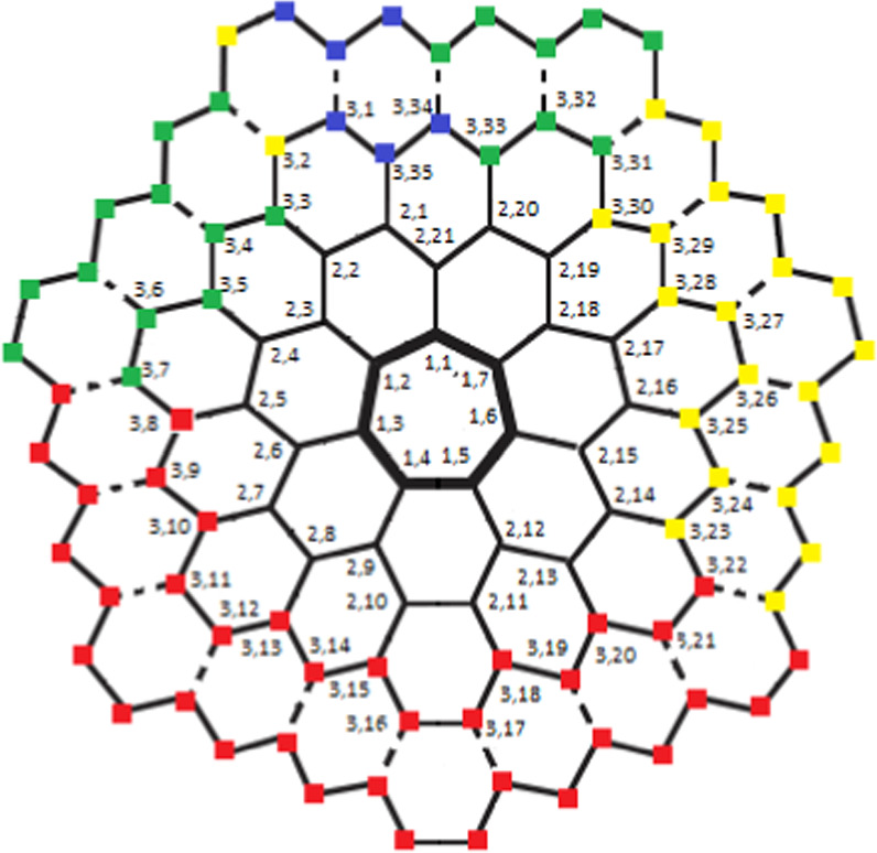
Figure 6. HCNs for Case 2.
Download figure:
Standard image High-resolution image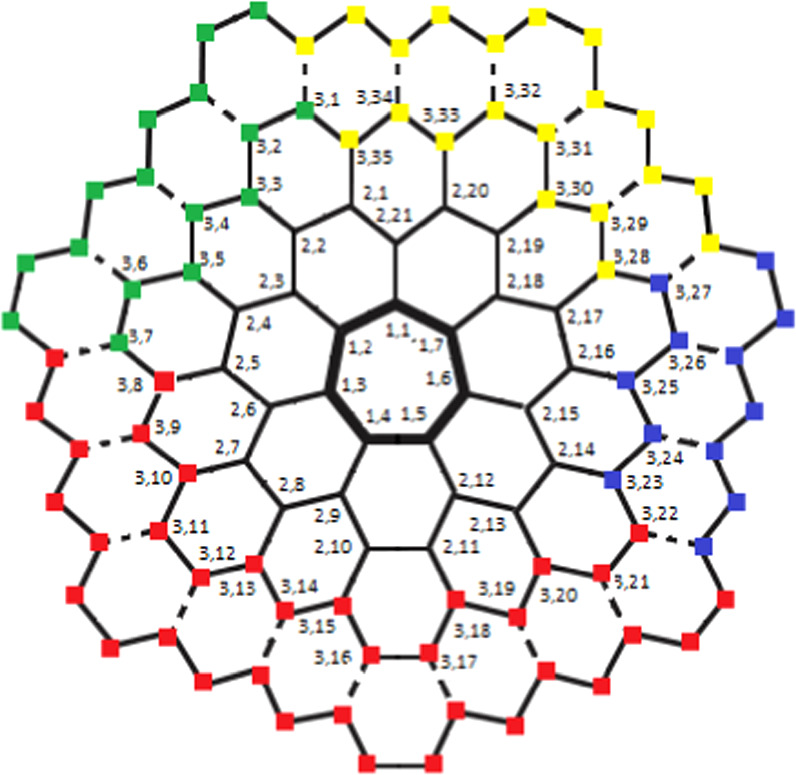
Figure 7. HCNs for Case 3.
Download figure:
Standard image High-resolution imageTable 6. When both the vertices in Hs lie on the same vertex cycle present in HCNs .
| Subcase | Resolving sets | Contradictions |
|---|---|---|
| 1 | Hs = {q1,1, q1,l }; b=1 & 7 ≥ l ≥ 2 | cv (q2,1∣Hs ) = cv (q2,20∣Hs ). |
| 2 | Hs = {qb,14b−7, qb,l }; s − 1 ≥ b ≥ 2 & 14b − 6 ≥ l ≥ 1 | cv (qb,1∣Hs ) = cv (qb,14b−8∣Hs ) or cv (qb,1∣Hs ) = cv (qb−1,1∣Hs ) or cv (qb−1,1∣Hs ) = cv (qb,14b−8∣Hs ) or cv (qb,8b−3∣Hs ) = cv (qb+1,8(b+1)−1∣Hs ). |
| 3 | Hs = {qb,1, qb,l }; b=s & 14b − 7 ≥ l ≥ 2 | cv (qb,1∣Hs ) = cv (qb,14b−8∣Hs ) or cv (qb,1∣Hs ) = cv (qb−1,1∣Hs ) or cv (qb−1,1∣Hs ) = cv (qb,14b−8∣Hs ) or cv (q1,6∣Hs ) = cv (q2,18∣Hs ). |
Table 7. When both the vertices in Hs lie on the two neighboring vertex cycle present in HCNs .
| Subcase | Resolving sets | Contradictions |
|---|---|---|
| 1 | Hs = {q1,1, qb,l }; b=2 & 21 ≥ l ≥ 1 | cv (q2,1∣Hs ) = cv (q2,20∣Hs ) or cv (q1,3∣Hs ) = cv (q2,3∣Hs ) or cv (q1,6∣Hs ) = cv (q2,18∣Hs ). |
| 2 | Hs = {qb,1, qb+1,l }; s − 1 ≥ b ≥ 2 & 14(b + 1) − 7 ≥ l ≥ 1 | cv (qb+1,1∣Hs ) = cv (qb+1,14(b+1)−8∣Hs ) or cv (qb+1,14(b+1)−7∣Hs ) = cv (qb,14b−7∣Hs ) or cv (qb,2∣Hs ) = cv (qb+1,14(b+1)−7∣Hs ) or cv (qb,2∣Hs ) = cv (qb,14b−7∣Hs ). |
Table 8. When both the vertices in Hs lie on two non-neighboring vertex cycles present in HCNs .
| Subcase | Resolving sets | Contradictions |
|---|---|---|
| 1 | Hs = {q1,1, qb,l }; s ≥ b ≥ 3 & 14b − 7 ≥ l ≥ 1 | cv (qb,1∣Hs ) = cv (qb,14b−8∣Hs ) or cv (qb,2b+1∣Hs ) = cv (qb,2b+3∣Hs ) or cv (qb,8b−3∣Hs ) = cv (qb,8b−5∣Hs ) or cv (q1,2∣Hs ) = cv (q2,1∣Hs ). |
| 2 | Hs = {qb,1, qc,l }; s − 2 ≥ b ≥ 2; s ≥ c ≥ b + 2 & 14b − 7 ≥ l ≥ 1 | cv (qb,2∣Hs ) = cv (qb,14b−7∣Hs ) or cv (qb,14b−7∣Hs ) = cv (qb+1,14(b+1)−7∣Hs ) or cv (qb,2∣Hs ) = cv (qb+1,14(b+1)−7∣Hs ) or cv (qb+1,1∣Hs ) = cv (qb+1,14(b+1)−8∣Hs ). |
From theorem 2, we find that  ; ∀
s ≥ 2 and from theorem 3, for HCNs
, we find that
; ∀
s ≥ 2 and from theorem 3, for HCNs
, we find that  ; ∀
s ≥ 2. Then, from these findings regarding the graph of HCNs
, we have the following result:
; ∀
s ≥ 2. Then, from these findings regarding the graph of HCNs
, we have the following result:
Theorem 4. For every  , we have
  .
.
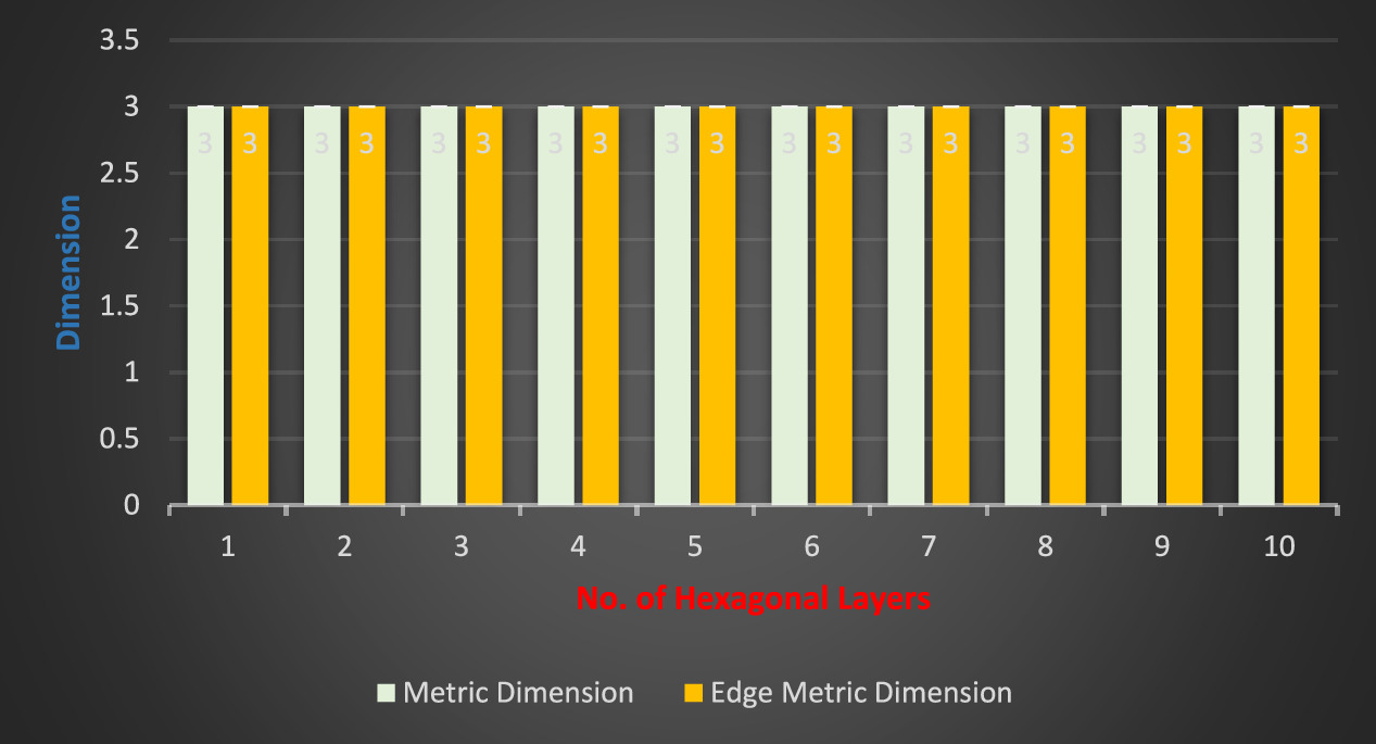
Remark 1. For the molecular complex graph of HCNs
, we find an interesting relation between MD and edge metric dimension [9] that,  . The comparison analysis between these two distinct resolving parameters for HCNs
is clearly provided in figure 8 and the value of MD and edge metric dimension does not depend upon the number of vertices present on any vertex-cycle of HCNs
.
. The comparison analysis between these two distinct resolving parameters for HCNs
is clearly provided in figure 8 and the value of MD and edge metric dimension does not depend upon the number of vertices present on any vertex-cycle of HCNs
.
Figure 8. The comparison plot for distinct resolving parameters in HCNs .
Download figure:
Standard image High-resolution image
5. Independent resolving number for HCNs
From the above findings regarding HCNs , we find that there exists a minimum RS Hs in HCNs with cardinality three. Now, the question arises: does Hs exhibit some other graph-theoretic properties or not? Thus, we explore some other properties for the minimum RS Hs , in particular, we determine that whether the set Hs is independent or not. Therefore, regarding the minimum resolving independent set (MRIS) Hs i in HCNs , we have the following result:
Theorem 5. For every  , the graph HCNs
has MRIS Hs
i
with cardinality 3.
, the graph HCNs
has MRIS Hs
i
with cardinality 3.
Proof. Similar to the proof of theorem 4.□
Example 5.1. Let us consider a set  , and fix s = 4 (see figure 2). Next, the metric representations for every member in
  corresponding to set H4 can be shown in table 9.
Table 9. When Hs = {q4,1, q4,3, q4,22} and s = 4.
| qi,j | MR codes | qi,j | MR codes | qi,j | MR codes | qi,j | MR codes | qi,j | MR codes |
|---|---|---|---|---|---|---|---|---|---|
| q1,1 | (6,6,9) | q1,2 | (7,5,8) | q1,3 | (8,6,7) | q1,4 | (9,7,6) | q1,5 | (9,8,7) |
| q1,6 | (8,8,8) | q1,7 | (7,7,9) | q2,1 | (4,4,11) | q2,2 | (5,3,10) | q2,3 | (6,4,9) |
| q2,4 | (7,5,10) | q2,5 | (8,6,9) | q2,6 | (9,7,8) | q2,7 | (10,8,7) | q2,8 | (11,9,6) |
| q2,9 | (10,8,5) | q2,10 | (11,9,4) | q2,11 | (11,10,5) | q2,12 | (10,9,6) | q2,13 | (11,10,7) |
| q2,14 | (10,10,8) | q2,15 | (9,9,9) | q2,16 | (10,10,10) | q2,17 | (9,9,11) | q2,18 | (8,8,10) |
| q2,19 | (7,7,11) | q2,20 | (6,6,11) | q2,21 | (5,5,10) | q3,1 | (2,2,13) | q3,2 | (3,1,12) |
| q3,3 | (4,2,11) | q3,4 | (5,3,12) | q3,5 | (6,4,11) | q3,6 | (7,5,12) | q3,7 | (8,6,11) |
| q3,8 | (9,7,10) | q3,9 | (10,8,9) | q3,10 | (11,9,8) | q3,11 | (12,10,7) | q3,12 | (13,11,6) |
| q3,13 | (12,10,5) | q3,14 | (13,11,4) | q3,15 | (12,10,3) | q3,16 | (13,11,2) | q3,17 | (13,12,3) |
| q3,18 | (12,11,4) | q3,19 | (13,12,5) | q3,20 | (12,11,6) | q3,21 | (13,12,7) | q3,22 | (12,12,8) |
| q3,23 | (11,11,9) | q3,24 | (12,12,10) | q3,25 | (11,11,11) | q3,26 | (12,12,12) | q3,27 | (11,11,13) |
| q3,28 | (10,10,12) | q3,29 | (9,9,13) | q3,30 | (8,8,12) | q3,31 | (7,7,13) | q3,32 | (6,6,13) |
| q3,33 | (5,5,12) | q3,34 | (4,4,13) | q3,35 | (3,3,12) | q4,1 | (0,2,15) | q4,2 | (1,1,14) |
| q4,3 | (2,0,13) | q4,4 | (3,1,14) | q4,5 | (4,2,13) | q4,6 | (5,3,14) | q4,7 | (6,4,13) |
| q4,8 | (7,5,14) | q4,9 | (8,6,13) | q4,10 | (9,7,12) | q4,11 | (10,8,11) | q4,12 | (11,9,10) |
| q4,13 | (12,10,9) | q4,14 | (13,11,8) | q4,15 | (14,12,7) | q4,16 | (15,13,6) | q4,17 | (14,12,5) |
| q4,18 | (15,13,4) | q4,19 | (14,12,3) | q4,20 | (15,13,2) | q4,21 | (14,12,1) | q4,22 | (15,13,0) |
| q4,23 | (15,14,1) | q4,24 | (14,13,2) | q4,25 | (15,14,3) | q4,26 | (14,13,4) | q4,27 | (15,14,5) |
| q4,28 | (14,13,6) | q4,29 | (15,14,7) | q4,30 | (14,14,8) | q4,31 | (13,13,9) | q4,32 | (14,14,10) |
| q4,33 | (13,13,11) | q4,34 | (14,14,12) | q4,35 | (13,13,13) | q4,36 | (14,14,14) | q4,37 | (13,13,15) |
| q4,38 | (12,12,14) | q4,39 | (11,11,15) | q4,40 | (10,10,14) | q4,41 | (9,9,15) | q4,42 | (8,8,14) |
| q4,43 | (7,9,15) | q4,44 | (6,8,15) | q4,45 | (5,7,14) | q4,46 | (4,6,15) | q4,47 | (3,5,14) |
| q4,48 | (2,4,15) | q4,49 | (1,3,14) |
6. Conclusion
Challenging applications pertaining to graph theory in order to solve molecular problems is a subject of the chemical graph theory (CGT). The key role of CGT is to depict the molecule's energy as an entire entity, including its orbital, electronic structures, molecular branching, structural fragments, and among other things, by reducing a molecule's topological structure to a single integer using computational invariants. These well-studied graph theoretic invariants are expected to correspond with empirically recorded physical observable, allowing theoretical predictions to be utilized to investigate chemical processes even for molecules that do not yet exist. Metric basis and RS for any simple connected graph are the graph-theoretic invariants that hold significant information to uniquely identify every member (vertices or/and edges) present in the graph under consideration. In this manuscript, we have studied the graph of HCNs
in terms of its vertex resolvability. In particular, we have investigated the minimum RS as well as a MB for the molecular complex graph of HCNs
. We proved that  ; ∀
s ≥ 2. Moreover, a comparison between MD and edge metric dimensions of HCNs
is provided as
; ∀
s ≥ 2. Moreover, a comparison between MD and edge metric dimensions of HCNs
is provided as  ; ∀
s ≥ 2. Finally, we showed that the minimum RS in HCNs
exhibits the property of independence. In the future, the other interesting variants of MD (i.e., mixed metric dimension, fault-tolerant metric dimension, partition dimension, etc.) for molecular complex graphs of HCNs
will be investigated [44, 45].
; ∀
s ≥ 2. Finally, we showed that the minimum RS in HCNs
exhibits the property of independence. In the future, the other interesting variants of MD (i.e., mixed metric dimension, fault-tolerant metric dimension, partition dimension, etc.) for molecular complex graphs of HCNs
will be investigated [44, 45].
Acknowledgments
We would like to express our sincere gratitude to the referees for their careful reading of this manuscript and for all of their insightful comments/criticism, which have resulted in several major improvements to this manuscript.
Data availability statement
The data cannot be made publicly available upon publication because no suitable repository exists for hosting data in this field of study. The data that support the findings of this study are available upon reasonable request from the authors.
Conflicts of interest
Authors have nothing to declare as conflict of interest.
Authors contributions
All authors contributed equally.
Funding
No funding was used in this study.