


Abstract
When light interacts with a material made from subwavelength periodically arranged constituents, non-local effects can emerge. They occur because of either a complicated response of the constituents or possible lattice interactions. In lowest-order approximations of a general non-local response function, phenomena like an artificial magnetism and a bi-anisotropic response emerge. However, investigations beyond these lowest-order descriptions of non-local effects are needed for optical metamaterials (MMs) where a significant long-range interaction becomes evident. This highlights the need for additional material parameters to account for spatial non-locality in an effective medium description. These material parameters emerge from a Taylor expansion of the general and exact non-local response function. Even though these non-local parameters improve the effective description, their physical significance is yet to be understood. To improve the situation, we consider a conceptional MM consisting of scatterers characterized by a prescribed multipolar response arranged on a square lattice. Lorentzian polarizabilities describe the scatterers in the electric dipolar, electric quadrupolar, and magnetic dipolar terms. A slab of such a MM is homogenized while considering an increasing number of non-local terms in the constitutive relations at the effective level. We show that the effective permittivity and permeability are linked to the electric and magnetic dipole moments of the scatterers. The non-local material parameters are related to the higher-order multipolar moments and their interaction with the dipolar terms. Studying the effective material parameters with the knowledge of the induced multipolar moments in the lattice facilitates our understanding of the significance of each material parameter. Our insights aid in deciding on the order to truncate the Taylor expansion of the considered constitutive relations for a given MM.
Export citation and abstract BibTeX RIS

Original content from this work may be used under the terms of the Creative Commons Attribution 4.0 license. Any further distribution of this work must maintain attribution to the author(s) and the title of the work, journal citation and DOI.
1. Introduction
Metamaterials (MMs) have a profound impact on our ability to control the propagation of light [1–6]. MMs consist (mostly) of periodically arranged scatterers, also called meta-atoms. In a stricter sense, we require the meta-atoms to be placed with a sufficiently sub-wavelength periodicity. This allows us to replace the complicated mesoscopic MM with a homogeneous medium. The homogeneous medium is characterized by effective material properties (EMPs) such that the electromagnetic fields propagate across macroscopic scales in the same manner as they would in the mesoscopic MM. A prime challenge for theoretical research is to develop an effective medium theory (EMT) that links the structured mesoscopic material to the macroscopic homogeneous one [7–11].
Historically, the basic concept behind an effective medium description dates back decades, when structured solid-state materials were described using an effective conductivity or permittivity [12–14]. These effective materials were characterized by the same material parameters at the qualitative level as their constituents but with quantitatively vastly different values. With the advent of more modern MMs, a strong focus has been dedicated to further developing EMTs that accommodate more exotic properties [9, 15–17]. Specifically, properties in the homogeneous material inaccessible with natural materials were at stake. An artificial magnetism at optical frequencies is a prototypical example [18–22]. But many more properties are relevant, e.g. bianisotropic, chiral, or, as we will see later, non-local properties.
By shifting our focus away from the general effective medium description, many attempts have been undertaken to gain a deeper insight into non-local effects. Non-locality, in general, can occur because of a higher-order multipolar response of the constituents that form the photonic material or from lattice interactions. In the context of MMs, it is often discussed in the context of spatially extended collective excitations characterized by a wave vector-dependent electromagnetic polarizability [23, 24].
In this context, zeroth-order spatial effects with  represent the local response of a medium, where long-wavelength approximations apply. Going further, it becomes apparent that bi-anisotropic responses result from light interacting with constituents having no inversion symmetry. This results from light probing spatial extents beyond a point-scatterer, thus identifying it as a non-local response. In essence, bianisotropy is a first-order non-local effect [16, 25, 26]. Much prior research has also been dedicated to exploring second-order non-local effects, such as artificial magnetism [27, 28]. In fact, a considerable body of literature has delved into non-locality up to this level [29–31], encompassing both natural materials and MMs. Moreover, when multiple scattering occurs among densely packed scatterers, it gives rise to complex interference effects, including phenomena like electromagnetically induced transparency [32] and the Brewster-like effect, where the absolute reflection coefficient reaches its minimum for a specific polarization [33]. Furthermore, concerning controlled near-field coupling, Fano resonances in plasmonic materials emerge from the interaction between superradiant and subradiant modes, introducing unique extinction features with characteristic narrow and asymmetric line shapes [34–36]. These examples further exemplify the diverse range of non-local effects within MMs. Notably, most of these effects fall within the lower-order approximation of the spatially dependent polarizability, categorizing them as weak spatial dispersion (WSD).
Besides the exotic MM properties, a strong spatial dispersion in the material properties motivated the community to investigate strong interactions among the meta-atoms [37–41]. It requires lending the meta-atoms a strong polarizability and packing them relatively densely. The emerging interactions among adjacent meta-atoms are commonly referred to as lattice interactions. Such strong interactions lead to a transfer of excitation across longer distances in the lattice, thus requiring a non-local description at the effective level [16, 42–44].
To accommodate these effects of non-locality, a non-local response kernel  can be used to express the constitutive relation in a homogenized MM as

Here,  is the electric displacement relating to
  the electric field through the distributional action over the whole MM volume v. Both depend on space. Moreover, the constitutive relation is written here in the temporal frequency domain. Hence, all quantities depend on the frequency ω or, alternatively, on the free space wavenumber
  .
.
Please note that equation (1) considers a homogeneous medium that extends infinitely. Naturally, such infinitely extended material does not exist. Nevertheless, it is a good starting point for a general theoretical discussion. The strategy here is rather generic and consists of two steps. In the first step, we need to identify the eigenmodes that can expand an arbitrary solution to Maxwell's equations in that material. In the second step, and when considering a space divided into finite domains occupied by different materials, interface conditions can be enforced to couple the solutions in the different spatial domains and to determine their exact amplitudes for a given illumination. Now, even though equation (1) is general and correct, it is challenging to use it in practice as especially the question of how to evaluate the convolution close to interfaces is hard to answer.
Therefore, to make practical use of such a constitutive relation, we approximate the general response function in Fourier space  by a Taylor expansion and retain only a few lowest order terms:
Here, the frequency-dependent Taylor coefficients  are the tensor-space representations of the material parameters in the spatial reciprocal space. A pictorial representation of the underlying idea is depicted in figure 1.

Figure 1. Pictorial representation of a non-local homogenization idea. Here, the periodic arrangement of the spherical scatterers represents the actual inhomogeneous MM with a periodicity Λ. An optical excitation, illustrated by the blue-colored cloud, emanates from the spheres but spreads across the entire MM. It is used to indicate a long-range interaction among the constituting scatterers. Towards the right, we see a transition into a homogeneous slab occupying the same spatial domain as the actual MM but hiding the inhomogeneity. This homogeneous slab shall be optically equivalent to the mesoscopic MM, and its properties are encoded in the effective material parameter tensors: ε, µ, γ, τ, etc up to an arbitrary order.
Download figure:
Standard image High-resolution imageIn the following, we restrict ourselves to centrosymmetric materials where the odd-order terms of the expansion vanish, i.e.  . Moreover, the expansion in figure 2 is unsuitable for general purposes since even for that general formulation, interface conditions cannot be identified [45]. These interface conditions, also known as additional boundary conditions, need to be known to study reflection and transmission from an interface and not just to consider light propagation in a homogeneous space. Possible additional interface conditions were only recently derived under the assumption that each term in the expansion above corresponds to a term where a specific material parameter is sandwiched between an equal number of
  operations [45]. In particular, we require that
and

hold.
Under this assumption, we write the constitutive relation in spatial Fourier domain as [46]
To ease the understanding of this equation, we have written each term in a dedicated line. The first term captures the permittivity  . That corresponds to the local electric response. The second term expresses the permeability
  , being a consequence of a WSD or weak non-locality. That is because even though it is a feature emerging from a higher-order term in a Taylor expansion of the response function for the electric field, it can be reformulated to appear as a local term in the response function of the magnetic field. Anticipating such a possible transformation, we have expressed the term in the electric response using the permeability. Finally, we consider two higher-order non-local material parameters
  and
and  .
.
In the past decade, advanced applications have emerged that exploit such a strong non-locality [47–52]. These developments have created a demand for suitable modeling approaches but, particularly, for a physical understanding of these terms. In other physical settings, an intuitive understanding of the effects of non-local interactions has already been developed [53, 54]. For acoustic MMs, for example, a pronounced interaction beyond the nearest neighbors, which can be deterministically controlled, gave rise to a roton-like dispersion relation [55, 56] for the lowest order mode. For such a roton-like dispersion relation, multiple eigenmodes can propagate at the same frequency in the lattice with different wavenumbers, offering effects such as negative refraction.
In this article, we attempt to draw an equivalent intuitive picture of the non-locality of electromagnetic MMs. In contrast to mechanical systems, electromagnetic unit cells cannot be connected physically, but rather, the lattice interaction has to be quantified. Herein, we study the emergence of higher-order non-local material parameters upon systematically homogenizing MMs made from meta-atoms with increasing complexity. To do so on phenomenological grounds, we need to control the multipolar contribution (i.e. position and width of the associated multipolar resonance) of the individual scatterer of the prospective infinite periodic array.
Based on [57], we describe the associated polarizabilities characterizing the scatterers with Lorentzian resonances, and we suitably choose the degrees of freedom in such a model. For simplicity, we consider isotropic scatterers arranged on a square lattice. This arrangement ensures inversion symmetry, leading to the response function  in the bulk so that the EMPs will be isotropic. By controlling the exact multipolar contents with increasing complexity, we study the impact of the electric and magnetic dipolar and the electric quadrupolar response on the effective properties.
To homogenize an MM made from such scatterers, we map the optical response of the actual periodic structure to that of the homogenized material characterized by a specific set of EMPs. For that, we rely on an approach where we consider the frequency- and angle-dependent reflection and transmission coefficients from a mesoscopic MM slab illuminated by a plane wave. The incident plane wave is TM-polarized, and the incidence angle is characterized by the x-component of the wave vector kx
. These reflection and transmission coefficients are inverted in a least-squares sense to provide effective material parameters. We achieve this through the gradient-based optimization procedure outlined in appendix
To elucidate the impact of each material parameter, we distinguish three different models for the constitutive relations with increasing complexity. These three models are: (i) the WSD, where the material is characterized only by permittivity and permeability, (ii) a first model that captures the effects of strong spatial dispersion (SSD), where the material is described additionally by the γ parameter, and we call it the γ model (SSD-γ), and finally (iii) a second model that captures effects of SSD where the material is described additionally by the τ parameter, and we call it the τ model (SSD-τ).
By homogenizing an MM made from scatterers with an increasingly more complicated multipolar response using different local and non-local constitutive relations, we aim to explore multiple aspects. First, by tracking the error we achieve for the different constitutive relations, we can quantify the advantage of non-local constitutive relations to homogenize a given MM [58]. Second, we approach the critical question of what these additional material parameters correspond to. Based on these insights, we can establish an idea of the upper bound for the truncation order in the Taylor series expansion of the response function equation (2) needed to homogenize a given MM. Finally, we also show that strong lattice effects impart higher-order multipolar moments in the bulk, thereby prompting to retain non-local effective material parameters to describe the considered MM at the effective level.
The manuscript is structured as follows. Section 2 provides technical details to describe the scatterers from which the MM is made. Afterward, the homogenization results with increasing complexity in the scatterers are discussed in section 3. We start with pure electric dipolar scatterers, continue with pure electric quadrupolar scatterers, and consider afterward scatterers characterized by a combination of different multipolar terms. We skip the consideration of a magnetic dipolar scatterer as it would duplicate insights obtained from the electric dipolar case. Finally, we conclude our findings in section 4.
2. Analytical model
To demonstrate the applicability of our homogenization models, we consider an MM made from a periodic arrangement of spherical scatterers with a predetermined multipolar response. We analyze three MMs made from meta-atoms with consecutively increasing complexities of supported multipole moments. We rely on the transition matrix formalism (T-matrix) method to design a meta-atom and compute the electromagnetic response of an MM. In this approach, the scattering properties of the meta-atoms are described by a matrix called the T-matrix. The T-matrix linearly relates the expansion coefficient of the incident fields (qe and qm for their respective electric and magnetic contributions) and the scattered fields (pe and pm for their respective electric and magnetic contributions), expanded in a vector spherical harmonic basis. The relation reads as:

The vectors p and q contain the expansion coefficients of scattered and incident fields, respectively, corresponding to their electric and magnetic parts. As these coefficients are a fundamental solution of the vector Helmholtz equations, access to the T-matrix guarantees the calculation of the scattered field of the meta-atom for any given incident field [59–61]. Additionally, to compute the complete scattering response of an MM made from periodically arranged scatterers, the algorithm from [62] is used. In this approach, the MM is assumed to be made by infinitely repeating identical copies of a meta-atom with a 2D periodicity. This assumption guarantees the validity of the translational addition theorem to be applied to the T-matrix describing the meta-atom, consequently allowing one to use the 2D Ewald summation, resulting in a rapidly converging solution determining the scattering response of the MM [63]. The outcomes of the algorithm are reflection and transmission coefficients from the MM for a given illumination.
Since the T-matrix can describe any unit cell irrespective of its shape and material, the choice of a spherical scatterer in this article is purely out of convenience. By choosing a spherical shape, we can use a Mie theory-based design strategy to describe the response from an individual scatterer [57]. Mie theory generally expresses the ratio between the scattered and incident fields in the Mie coefficients an and bn for the electric and magnetic contributions, respectively, where n refers to the multipolar order. This implies that the T-matrix can also be defined by these Mie coefficients. This is a convenient design approach because the Mie coefficients can be related to the polarizabilities of an isotropic particle [64] as


Here,  and
and  are the corresponding polarizabilities for the
  multipolar order. At this point, we can define the scattering properties of our meta-atom with a Lorentzian-type oscillator in the polarizability
  that reads as
where  is the resonance frequency of the oscillator,
  is the oscillator strength that determines the width of the resonance, and
  is the associated Ohmic loss with the dimension of
 ![$[T^{-1}]$](https://content.cld.iop.org/journals/1367-2630/25/12/123014/revision2/njpad1010ieqn22.gif) . The labels
. The labels  refer to the electric and magnetic contribution and
  to the multipolar order.
In this way, predetermined Lorentzian polarizabilities for the individual nanosphere can be directly considered in the T-matrix that expresses the scattering response of one sphere. For example, below is the T-matrix of size  describing the pure electric and magnetic dipolar sphere at some frequency ω:
The choice of spherical symmetry for the meta-atoms further simplifies the T-Matrix to have only diagonal entries. This method can be adapted to include arbitrarily higher multipolar orders—limited only by the available computational resources—by simply adding the corresponding Mie coefficients to the diagonal.
Relying on this T-matrix method, a freestanding square array of spherical scatterers is built with a periodicity Λ. The associated reflection  and transmission
  coefficients are calculated for all considered frequencies ω upon plane wave illumination. The incident field is TM-polarized. The incidence angle of the illuminating plane wave can be controlled by changing the x-component of the wave vector kx
of the incident field. This set of reflection and transmission coefficients is the referential data considered in the subsequent parameter retrieval.
coefficients are calculated for all considered frequencies ω upon plane wave illumination. The incident field is TM-polarized. The incidence angle of the illuminating plane wave can be controlled by changing the x-component of the wave vector kx
of the incident field. This set of reflection and transmission coefficients is the referential data considered in the subsequent parameter retrieval.
3. Results and discussion
This section is divided into three subsections. In these subsections, we discuss an MM made from a purely electric dipolar scatterer, a purely electric quadrupolar scatterer, and a scatterer that sustains an electric dipole and quadrupole moment and a magnetic dipole moment, respectively. First, we homogenize each MM, considering the three different constitutive relations. One of them is local, and the other two are non-local. Then, we will judge with a suitably chosen objective function how well these constitutive relations can describe the MM at the effective level. The higher-order non-local constitutive relations perform, naturally, better. We also discuss the dispersion in the effective material parameters. This analysis allows us to judge in which order we can truncate the Taylor expansion of the constitutive relation to homogenize an MM made from scatterers with an increasingly more complicated multipolar response.
3.1. Pure electric dipole scatterer
As our first example, we model the particle as a pure electric dipole surrounded by air. The polarizability is characterized by a resonance frequency of  , oscillator strength of
 , and the absorption in the particle is given by the Ohmic loss factor
  . The associated characteristic polarizability is shown in figure 2(a). We further assume a periodic arrangement of such spheres along a square lattice with a periodicity of
  . To further ensure isotropy, particularly along the normal direction, the thin film is simulated with a thickness matching the same periodicity Λ. We move forward by homogenizing this MM along the lines described above. For the homogenization, we consider the three different constitutive relations separately.
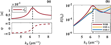
Figure 2. (a) Amplitude and phase of the electric dipolar polarizability of the sphere considered in the initial example. (b) Error function plotted in logarithmic scale as a function of frequency k0 when homogenizing the MM made from a periodic arrangement of these electric dipolar spheres into a lattice with a period of  nm. The error function is shown when homogenizing the MM using the WSD model (red), the SSD-γ model (yellow), and the SSD-τ model (blue). The gray shaded area marks the frequency domain, where the homogenization is unreliable because of an emerging anisotropy. The black dashed vertical line represents Lorentzian resonance at frequency
  for the isolated particle.
Download figure:
Standard image High-resolution imageThe starting point of our analysis is to judge the quality of the equivalent effective medium obtained by each of the considered homogenization models. The quality is considered as the ability of the homogenized material to provide the same optical response as the actual mesoscopic MM. To do so, we define the error function
that compares the optical coefficients, i.e. reflection R and transmission T, of the actual MM with the predictions from each model. Furthermore, we employ an optimization algorithm that formulates the error function  using our forward solver for a set of ranges of randomly chosen initial material parameters. The effective material parameters are then iteratively determined through a least-squares minimization procedure, such that
  is minimum appendix
Figure 2(b) shows the prediction error of all models in logarithmic scale as a function of frequency k0. The shaded region corresponds to frequencies where the influence of symmetry breaking in the third dimension is strong, making the system less isotropic and, hence unable to be homogenized. The breaking of the symmetry results from considering only a single MM layer and not a stacked version. It causes the component of the effective material parameters in the direction normal to the interface to be different from the components in transverse directions.
To estimate any deviation from isotropy, we examine the T-matrix of the particle making up the considered one-layer MM in the Cartesian basis. For the expected isotropic structure, we require that the Mie coefficients in the  directions be identical across the considered frequency spectrum k0. In turn, we exclude those frequencies that fail to maintain isotropy (shaded region in figure 2(b)). While we can discuss the results in this spectral domain, they must be taken carefully as they are influenced by the consideration of just a single-layer MM.
From figure 2(b), it can be seen that the WSD model performs worse than both SSD models. The error is larger across all frequencies where homogenization is reasonable. In particular, close to the resonance frequency of the sphere from which the MM is made, the homogenization of the MM using the WSD is worse. That is not surprising, given that the critical length scale of  is only slightly smaller, not significantly so. This results in the lattice behaving as if the scatterers were densely packed relative to the wavelength, resulting in a robust long-range interaction. Consequently, the resonance causes a non-local spread of excitation across the lattice that requires a non-local constitutive relation to capture it. This initial insight shows the advantage of using a non-local constitutive relation over the conventional WSD model to homogenize even such a basic MM.
In figure 3, we show the real and imaginary parts of the effective material parameters retrieved using the WSD and the SSD models for the considered electric dipole example. To ensure passivity throughout the article, we explicitly constrain the imaginary component of the electric permittivity to be positive ( ) in the retrieval process. Firstly, we observe in figure 3 that all three homogenization models predict a Lorentzian resonance in the electric permittivity ε. This is no surprise since we have considered an electric dipolar meta-atom. We also observe the emergence of a weak anti-resonance in the permeability µ. Qualitatively, the dispersion in these material parameters remains the same for all three constitutive relations. Still, the magnitude slightly changes from the WSD to the SSD models.

Figure 3. Effective material parameters retrieved within WSD-γ model (red), the SSD-γ model (yellow), and the SSD-τ model (blue) as a function of the frequency k0. Here, an MM was considered made from a periodic arrangement of spheres characterized by an electric dipolar response. The gray shaded area marks the frequency domain, where the homogenization is unreliable because of an emerging strong anisotropy.
Download figure:
Standard image High-resolution imageSecondly, the difference between the values for the ε and µ parameters is relatively small for the SSD models. The additional consideration of a first non-local term in the SSD-γ model is necessary to improve our ability to homogenize the MM, but it has no substantial effect. Higher-order non-local terms are not required to be considered. That complements observations in figure 2(b), where it is shown that the SSD-γ model (yellow curve) and the SSD-τ model (blue curve) homogenize the MM equally well. The error function is nearly identical when the MM is homogenized with both possible constitutive relations. Moreover, using the SSD-τ model, the τ parameter takes negligible values and does not impact the optical coefficients. The algorithmic procedure used in the retrieval causes some non-zero values in the τ-parameter, but it has no notable impact on the optical coefficients. It implies that the additional τ parameter is redundant, and the SSD-γ model is already sufficient to accommodate the lattice interactions arising among the dipolar meta-atoms.
Obviously, for such a basic system, the results might look intuitive. Therefore, we increase the complexity of the lattice interaction by describing the individual scatterer with a higher multipolar order in the following.
3.2. Pure electric quadrupolar scatterer
In efforts to push the limits of the SSD-γ model, we now consider a pure electric quadrupolar (EQ) scatterer from which the MM is made. Based on the theory of current multipoles, each EQ can be decomposed into two copies of electric dipolar current with a phase shift of π between each pair [65]. Similarly, it is also understood that a substantial increase in the quadrupolar excitation in any periodic system significantly affects the magnetic permeability tensor [66–68]. Therefore, we assert that an EQ reflects the strength of a certain configuration of point dipoles. Thus, prompting the need for higher-order spatial derivatives of the electric field tensor for describing the full response of the periodic system.
Comparable to the previous subsection, we design the spherical scatterer to have a Lorentzian polarizability ( ) with a resonant frequency at
  , oscillator strength of
  , and the absorption in the particle is given by the Ohmic loss factor
  . To describe this polarizability as an EQ, the T-matrix of the isolated particle is constructed in the angular momentum basis. Then Mie coefficients (aq
) corresponding to
. To describe this polarizability as an EQ, the T-matrix of the isolated particle is constructed in the angular momentum basis. Then Mie coefficients (aq
) corresponding to  are contained in the angular momentum j = 2 matrix components (for this example, the dipolar components (j = 1) are set to zero). The corresponding MM has a periodicity set to
  .
.
Following the above procedure, we homogenize the MM using the three constitutive relations and study the error function. Results are shown in figure 4(b), where the error function depending on the frequency on a logarithmic scale is plotted. The curve corresponding to the WSD model performs poorly compared to the SSD models and fails to show any significant features pointing toward a possible resonance. Furthermore, when compared with the corresponding WSD results from the ED example (figure 2), the error increased by one order of magnitude across the considered frequency spectrum. This can be attributed to the very high amplitude of the pure EQ contribution to the overall response of the system compared to that of the induced quadrupolar moments in the ED example. The WSD model is obviously unable to capture the response of such MMs made from EQ scatterers at the homogeneous level.

Figure 4. (a) Amplitude and phase of the electric quadrupolar polarizability of the sphere considered in the second example. (b) Error function plotted in logarithmic scale as a function of frequency k0 when homogenizing the MM made from a periodic arrangement of these electric quadrupolar spheres into a lattice with a period of  . The error is shown when homogenizing the MM using the WSD model (red), the SSD-γ model (yellow), and the SSD-τ model (blue). The gray shaded area marks the frequency domain, where the homogenization is unreliable because of an emerging strong anisotropy. The black dashed line represents Lorentzian resonance at frequency
  for the isolated particle.
Download figure:
Standard image High-resolution imageIn contrast, both SSD models predict the optical coefficients across the entirely considered spectral range an order of magnitude more accurately than the WSD model. Furthermore, for frequencies  (corresponding to longer wavelengths, λ), the error function is consistently smaller when homogenizing the MM with the SSD-τ model when compared to the SSD-γ model. It turns out that the long-range lattice interactions in that specific example are captured better when using a higher-order non-local constitutive relation such as the SSD-τ model.
Indeed, at this point, one further needs to examine the retrieved effective material parameters to judge the impact of these additional material parameters quantitatively. In figure 5, we show the real and imaginary parts of the effective material parameters as retrieved from both SSD models as a function of frequency. With the WSD model, the optimizer finds no good solution for the  component. Moreover, the
  saturates close to zero, revealing a tendency to move into the negative quadrant, which was excluded from the constraint imposed.
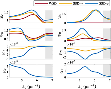
Figure 5. Effective material parameters for an MM made from a periodic arrangement of spheres characterized by an electric quadrupolar response retrieved within the WSD-γ model (red), the SSD-γ model (yellow), and the SSD-τ model (blue) as a function of the frequency k0. The gray shaded area marks the frequency domain, where the homogenization is unreliable because of an emerging strong anisotropy.
Download figure:
Standard image High-resolution imageOn using the SSD-τ model, a significant re-normalization happens of the non-local parameter γ. In contrast, the electric permittivity ε and magnetic permeability µ show minimal changes from their values calculated using the SSD-γ model. This contrast in the value of γ changes the optical coefficients and, therefore, improves the error function  .
.
An additional observation on the retrieved material parameters using the SSD-τ model is that, towards the smaller frequencies in figure 5, the real part of the permittivity ( ) approaches unity, while the imaginary part (
 ) approaches zero. This behavior indicates that the permittivity is approaching the value of vacuum permittivity, as expected in the absence of an electric dipole. Furthermore, the presence of the electric quadrupolar scatterer in a lattice can significantly affect the overall magnetic response of the medium, which is captured by the magnetic permeability µ within the effective medium theory. Thus, the effective magnetic permeability
  does not display any decay to the value of vacuum permeability. Finally, any long-range interactions among the scattering particles in the original MM are reflected in the values of non-local parameters γ and τ at lower k0 values.
Next, we analyze the impact of the EQ on the non-local material parameter τ. For that purpose, we modify the oscillator strength  as given in figure 6(a) and study its impact on the EMPs. Here, the polarizability phase φ is maintained for all values of
  . Therefore, the variation is purely in the amplitude
  of the EQ. During this analysis, the parameters for the scatterers that compose the MM except
  in equation (8) have been maintained from the example shown in figure 4.
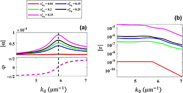
Figure 6. (a) Amplitude and phase of the electric quadrupolar polarizability of the sphere considered in the second example but with a modified oscillator strength  . The black dashed vertical line represents Lorentzian resonance at frequency
  for the isolated particle (b) The absolute value of the effective material parameter τ from the retrieval as a function of the oscillator strength
  in the considered frequency range.
Download figure:
Standard image High-resolution imageThe results are shown in figure 6(b). Here, the absolute values of the effective τ as a function of frequency are illustrated when considering a different strength of the electric quadrupole moment. Evidently,  grows with the increasing contribution from the EQ. As hypothesized, an increased EQ contribution requires at least the SSD-τ model to describe its optical properties in the effective medium description.
From the previous two examples, we can safely generalize that the relevance of the choice for the homogenization model depends on the multipolar order of the MM.
3.3. Spherical scatterer with a combination of multipoles
To study a more advanced example, we consider an MM made from spherical scatterers described by a combination of different resonant multipolar contributions. The Lorentzian polarizabilities describing the isolated sphere are the electric dipole  , magnetic dipole
  , and electric quadrupole
  . They all share a Lorentzian type resonance centered at the frequency
  . The associated oscillator strength of
  , given in the order electric dipole, magnetic dipole, electric quadrupole, and the damping parameter is maintained at a constant value of
  for all the considered moments.
Figure 7(a) shows the amplitude and shared phase of the respective multipolar polarizabilities. Since the resonance frequency and the damping parameter are the same for all multipole moments, the polarizabilities share the same phase and only differ in amplitude. In this setting, the combination of multipolar contributions to the response sustained by each scatterer introduces strong interparticle coupling. This coupling causes a strong non-local interaction among the scatterers across the considered frequency range.

Figure 7. (a) Amplitude and phase of the polarizabilities of the sphere considered in the third example. The sphere is characterized by an electric dipole ( ), electric quadrupole (
 ), and magnetic dipole (
 ) moment. The polarizabilities share the same resonance frequencies at
  and differ only by their oscillator strength. (b) Error function plotted in logarithmic scale as a function of frequency k0 when homogenizing the MM made from a periodic arrangement of spheres characterized by an electric dipolar, magnetic dipolar, and electric quadrupolar response into a lattice with a period of
  . The error function is shown when homogenizing the MM using the WSD model(red), the SSD-γ model (yellow), and the SSD-τ model (blue). (c) Absolute values of the reflection (R) and (d) absolute values of the transmission (T) as a function of frequency (k0) and incidence angle (θ) of the actual MM made from the periodic arrangement of these spheres. The period is chosen to be, again,
  .
.
Download figure:
Standard image High-resolution imageTo visualize the strong interaction among the multipoles, we show the absolute reflection and transmission in figures 7(c) and (d) as a function of frequency k0 and incidence angle θ calculated for the actual MM using the full-wave Maxwell solver. We are specifically interested in capturing with the effective description details such as  at lower frequencies (longer wavelengths) and angles beyond the paraxial limit. In figure 7(c), spectral sharp features at some frequencies and some angles indicate the presence of resonances, highlighting the signatures of a strong non-locality. Similarly, in figure 7(d), we notice that the main resonant features of the infinite periodic array redshift from the resonance frequency of the isolated particle (dashed line), showing strong lattice interactions. This configuration manifests a strong interaction among the intrinsic multipole moments resonating at the same frequency [69]. Therefore, it is a great example to probe for the limits of all three considered homogenization models.
We postulate that any prominent interactions among the scatterers coming from the ED contribution should be captured by the SSD-γ model. We do so because, in the initial example, we already observed that the additional consideration of the non-local τ parameter did not improve the description of a pure electric dipolar lattice. With the additional presence of the intrinsic EQ and the MD, we posit that further higher-order interactions among the multipoles have to be accounted for by the τ parameter.
We again start our discussion by judging the quality of the error function obtained from all three homogenization models. Figure 7(b) carries the error function in the logarithmic scale depending on the frequency. Immediately, we see the WSD model (red curve) performs poorly, especially toward higher frequencies. On comparing with the results from the SSD models, both the SSD models outperform the WSD model by at least two orders of magnitude. These observations conclusively dictate that as the complexity of the multipolar moments describing the MM increases, the WSD model is unreliable and should be disregarded for describing complex MMs within the homogeneous framework.
Having said that, we further quantify the improvements of non-locality offered by the SSD models (yellow and blue curves). From these curves, we clearly see reduced values for the error function when using the non-local constitutive laws for the effective description of the MM. Specifically, at very small frequencies  (at longer wavelengths), the SSD-τ model surpasses the SSD-γ model. This observation immediately reveals the necessity of the SSD-τ model in homogenizing the considered MM and, therefore, predicting a more realistic effective medium description. One should, therefore, use the SSD-τ model to retrieve the right effective material parameters and the associated optical coefficients.
In the following, we further discuss the retrieved effective material parameters and their prediction of the reflection and transmission coefficients for each of the considered homogenization models.
We show in figure 8 the retrieved effective material parameters using the three different constitutive relations. Please note, to see the fine features in the EMP, we normalized the non-local parameters by the corresponding powers of k0 in the insets. Here, we first study the SSD models to incur their advantage over the conventional WSD models. Both the SSD-γ and SSD-τ models predict similar trends for the electric permittivity ε and magnetic permeability µ. A Lorentzian type resonance for both parameters indicates the presence of the resonating electric (ED) and magnetic dipolar (MD) contribution at a frequency close to the isolated resonant frequency  . The influence of the intrinsic electric quadrupolar moment (EQ) and its interaction with the other multipolar moments significantly re-normalizes the electric permittivity ε by imparting a redshift with respect to the prediction from the WSD model towards
  . Furthermore, the γ, corresponding to the SSD-γ and the SSD-τ model, estimates the shift in the resonance frequencies further away from
  , predicting the blue shift for the resonance frequency of the infinite periodic array as given in figure 7(d). Additionally, the SSD-τ model also predicts few additional features at frequencies beyond
  . By including τ in the constitutive relation, we see that other material parameters get re-normalized, introducing some additional features towards the tail end of the Lorentzian for the magnetic permeability µ and also for the γ. These additional features can be postulated as a consequence of some long-range lattice interactions, additionally inducing a vague magnetic response to the material. This detail goes missing if one restricts the constitutive relation to either WSD or the SSD-γ models.

Figure 8. Effective material parameters retrieved within the WSD model (red), the SSD-γ model (yellow), and the SSD-τ model (blue) as a function of the frequency k0. Here, an MM was considered made from a periodic arrangement of spheres characterized by an electric dipolar, electric quadrupolar, and magnetic dipolar response as shown in figure 7(a). Additionally, to appreciate some sharp features carried by the non-local material parameters, we include insets with the same data but where the y-axis of both γ and τ parameters are scaled by powers of frequency k0 (i.e.  and
and  ).
).
Download figure:
Standard image High-resolution imageFurther, to appreciate the physical significance of the SSD models, we also comment on the predictions obtained using the conventional long wavelength approximation of the constitutive relations (WSD models). The  and
and  from the WSD model rightly predict the expected Lorentzian signature showing the presence of the electric and magnetic dipole but with an apparent shift in the resonance frequency away from
  . On comparing the prediction from the SSD models, the effective
  and µ fail to incorporate effects from the strong interactions among the meta-atoms. For instance, the
  from the WSD model only shows the presence of the intrinsic magnetic dipole and does not account for the lattice-induced magnetic contributions. Furthermore, the curves for
  conclude that the long wavelength approximation once again fails to predict any conclusive fit when we require a positive
  . Judging by the values of
  , we assume that the WSD model can find a slightly better fit when
  would have been admitted.
So far, we have seen that the effective material parameters carry the signature of the underlying physical effects that characterize the considered particle arrangement. Next, we use these retrieved effective material parameters to predict the optical coefficients of the considered MM. The conclusions derived from the nature of material parameters also hold for the optical coefficients given in the 2D plots of figure 9. This figure shows the absolute values of the reflection coefficient as a function of frequency k0 and angle of incidence ![$\theta \in (0, 89^\circ]$](https://content.cld.iop.org/journals/1367-2630/25/12/123014/revision2/njpad1010ieqn93.gif) corresponding to the parameters retrieved in the WSD, SSD-γ, and SSD-τ model, respectively. These predictions shall be compared to full-wave simulations already shown in figure 7(c).
corresponding to the parameters retrieved in the WSD, SSD-γ, and SSD-τ model, respectively. These predictions shall be compared to full-wave simulations already shown in figure 7(c).
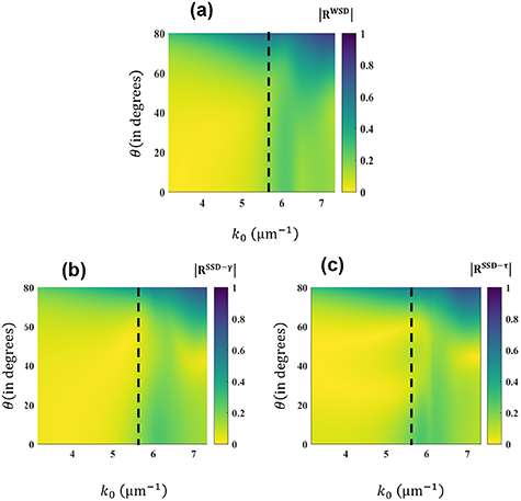
Figure 9. The absolute value of reflection as a function of frequency k0 and incidence angle θ shown in (a) for the WSD model, in (b) for the SSD model, and in (c) for the SSD
 model. These predictions shall be compared to full-wave simulations already shown in figure 7(c).
Download figure:
Standard image High-resolution imageHere, we concentrate on the discussion of features below the resonance frequency of the isolated particle  and at angles, θ from 30∘ to 75∘, to focus specifically on the beyond nearest-neighbor interactions. In the reference reflection coefficient, figure 7(c), we observe two sharp curves in the reflection spectral values across
  . Such prominent features remain missing in figures 9(a) and (b), indicating that both the WSD and the SSD-γ model fail to account for some long-range effects and interactions. Nonetheless, as we approach
  , a sharp dip in the reflection coefficient predicted by the SSD-γ model appears. The trend conveniently overlays with the plot for SSD-τ in figure 9(c). We also see that the error plots, as given in figure 7(b), show a small frequency interval where no particular advantage of using the SSD-τ model is observed. Additionally, tracing back these observations to the material parameters in figure 8, explains this feature as a dipole-like signature with ε values overlapping for both the SSD models. This observation concludes that the γ model limits itself within the effects up to the first-order approximation of the effective quadrupolar polarizability thereby predicting only the pure dipolar resonances found in figure 9(c) near
  . Furthermore, in figure 9(c), as concluded above from the optimized material parameters, the non-local parameter τ re-normalizes the other parameters, thereby accounting for the long-range interactions observed as sharp features in the predicted reflection coefficient at frequencies below the isolated resonant frequency capturing many prominent features as observed from the target reflection coefficient given in figure 8(c). This, in turn, improves the quality of the predicted optical coefficients, reducing the error function to a minimum.
Nevertheless, picking on the details reveals further very interesting observations. A closer look into the predicted optical coefficients reveals the inadequacy of the SSD-τ model. Exemplarily, figure 10 depicts the angular dependent reflection and absorption plus transmission for a selected free space wavelength of  . This wavelength is specifically highlighted because, here, the material shows a Brewster-like effect where the absolute reflection coefficient goes to its minimum. Such an effect is caused by complex interference effects among the multipolar moments [33] and hence a good representation of non-local interaction. Given the prior understanding of the nature of the material parameters obtained, we infer from figure 10(a) that, as expected, both the WSD and SSD-γ models are inferior to the SSD-τ model in capturing the sharp Brewster-like effect. This is because the SSD-τ model captures relatively correctly the sharp features at small angles of incidence. Furthermore, this trend remains consistent in moving closer to the frequency of the isolated particle resonance, as inferred from the error plot figure 8(b). Also, from figure 10(a), it is revealed that the SSD-τ model underfits the Brewster angle and thereby falls behind in predicting the right Brewster angle. Since this feature happens at a longer
  ratio, we proclaim that this effect hails from a long-range interaction which the SSD-τ model falls insufficient to account for and demands further higher-order material parameter to be considered to probe high-resolution field gradients.

Figure 10. Absolute reflection coefficient  and the absolute value of absorption and transmission coefficient (
 as a function of incidence angle for a wavelength of
  ).
).
Download figure:
Standard image High-resolution image
4. Conclusion
In this article, we explore the necessity of non-local constitutive relations to homogenize MMs. Furthermore, we explain the importance of each effective material parameter in describing strong lattice effects that manifest as a non-local response. As described by scattering theory, non-localities result from lattice-induced multipolar interactions. Therefore, a strong non-locality can be understood as strong lattice effects imparting higher-order multipole moments in the bulk. By homogenizing these MMs, we implicitly study the impact of these lattice-induced higher-order multipoles on the effective material parameters to describe the considered MM at the effective level.
We broadly answer two major questions regarding non-local homogenization methods. Firstly, we show that each of the material parameters considered in the system has a physical origin. By considering the geometrical symmetry of the considered optical structure, we show here that each effective material parameter has a signature of either the intrinsic multipolar moments or their strong interaction among the multipoles along the lattice. This feature elevates the importance of these additional material parameters and further opens a direction to explore this new degree of freedom sensibly. By choosing three examples with increasing multipolar complexity, we systematically study the effective material parameters as an equivalent representation of the induced multipolar moments and their interactions.
Along these lines, we see that the WSD model consistently underfits the optical response, thereby retrieving effective material parameters that are insufficient to describe the complete wave properties of the actual MM within the effective medium description. In contrast, the SSD models sufficiently capture many long-range wave interactions. The reduced error on using the SSD-γ and the SSD-τ, especially for lower frequencies, shows the reliability of using these models to homogenize non-local interactions for the considered MM examples effectively. Moreover, for a fixed periodicity, the significance of the non-local parameters strongly depends on the type of meta-atoms used to construct the MM. This statement is validated by tracking the importance gained by τ in describing systems with at least an electric quadrupolar moment.
Systematically considering each homogenization model separately reveals the re-normalization of the lower-order material parameters when an additional (significant) higher-order parameter is introduced into the constitutive relation. This observation is crucial for the examples with intrinsic EQ polarizabilities, as the inclusion of τ in the constitutive relation reveals a vague magnetic effect in the corresponding µ, otherwise hidden.
Secondly, we observe that the non-local parameter τ gains importance with the increasing complexity of multipoles describing the meta-atom. This, in turn, suggests that a simple scattering analysis of the meta-atom would assist in qualitatively judging the truncation order of the considered constitutive relation. On exploring the polarizability model of the constitutive relation, a rule of thumb is to have at least the SSD-γ model for a pure mesoscopic dipole system, and any signature of intrinsic quadrupole moment requires at least the SSD-τ model. Therefore, with prior knowledge about the multipolar moments excited in the meta-atom and a means to study the induced moments in the original MM, it is possible to have an educated guess on the truncation order for the considered material system.
A plausible extension of the study would be to establish a direct connection with scattering theory and formulate elegant expressions to express the non-local constitutive relation as a consequence of a complete multipolar description in bulk. This might allow for the explicit expression of the effective properties as a function of the scattering properties of the unit cell from which the MM is made and the consideration of the renormalization due to the interaction with all the particles in the lattice. Such a more explicit expression of the material properties would alleviate the need for a fitting procedure but would permit the direct expression of the effective properties. Moreover, the current interface conditions are applicable for planar interfaces only. It remains an open and interesting question to explore how they could be modified when considering curved interfaces. Alternatively, one could explore up to which curvature the deviation from a planar interface introduces only a minor error. This could open new perspectives in exploring the details of a non-local material response in the MMs in the presence of edges, defects, or disordered structures, where the effects of a non-locality should appear much more pronounced.
Acknowledgments
R V, F G, M P, and C R gratefully acknowledge financial support by the Deutsche Forschungsgemeinschaft (DFG, German Research Foundation) through Project-ID No. 258734477 - SFB 1173. Y A and C R acknowledge support by the German Research Foundation within the Excellence Cluster 3D Matter Made to Order (EXC 2082/1 under Project Number 390761711) and by the Carl Zeiss Foundation. The calculations in this work were performed on the HoreKa supercomputer funded by the Ministry of Science, Research and the Arts Baden-Württemberg and by the Federal Ministry of Education and Research. B Z and C R acknowledge support by the KIT through the 'Virtual Materials Design' (VIRTMAT) project. We want to thank Maria Paszkiewicz for designing the opening image of this article.
Data availability statement
All code for the parameter retrieval is made freely available under https://github.com/tfp-photonics/dinomat. All code for the optical simulations is made freely available under https://github.com/tfp-photonics/treams. This includes the reflection and transmission data used for generating the effective material parameters as shown in figures 3, 5, and 8.
The data that support the findings of this study are openly available at the following URL/DOI: https://github.com/tfp-photonics/dinomat.
Author contributions statement
R V, Y A, B Z, and C R conceived the numerical experiments and analyzed the results, M P and F G conceived the analytical developments. All authors reviewed the manuscript.
Appendix A: Effective parameter retrieval method
Instead of calculating the optical response of a certain set of constitutive parameters, one is often interested in the inverse problem, i.e. retrieving effective constitutive parameters given some optical response as can be obtained by, e.g. ellipsometric measurements. In this work, we consider simple geometries with known T-matrices from which we calculate reflectance and transmittance spectra over various incidence angles. From this data, we now seek to obtain a set of effective material parameters using the models presented in this work that yield a similar optical response. This means we are looking to minimize the difference between a target spectrum and that of the spectrum obtained by our models, which essentially describes a (nonlinear) least-squares problem.
Starting from a random (bounded) initial guess for the material parameters, we calculate the reflectance and transmittance at a specific k0 for all angles of incidence. The residuals of these values with those of some target reflectance and transmittance spectrum are then passed to a least-squares solver as implemented in SciPy [70] with a smooth L1 loss function:

where  is the residual vector defined by our error function in equation (10).
The forward solver is implemented using JAX [71] to enable JIT-compilation and automatic differentiation. The latter enables us to provide fast and accurate Jacobians to the optimization, which significantly speeds up convergence and ensures high-quality results. We allow for multiple restarts, i.e. we restart the fitting procedure from different initial guesses until a sufficiently small final error is reached. In practice, however, we have found that for many problems, a single trial is enough, and no restarts are needed.
After a set of material parameters for a specific k0 is found, the optimization moves to the next closest k0 (depending on discretization). To ensure smoothness in the constitutive relation and speed up convergence, the optimized material parameters of the previous iteration are taken as the initial guess for the current k0. This procedure is then repeated for all k0, resulting in the final constitutive relation for all material parameters under consideration (i.e. the procedure is the same for all models discussed herein).
Appendix B: Forward solver for the homogeneous medium
This section outlines the computations employed in assigning the optimized effective material parameters to the homogeneous equivalent of the actual MM.
We first introduce here the working of our in-house forward solver. The first step in using the solver is to select the preferred homogenization model. Based on the nature of the terms in equation (4), we divide the dispersion relations into three models using the general constitutive relations discussed in equation (4). The weak spatial dispersion model (WSD) describes the homogeneous slab with only the local material parameters: electric permittivity ɛ and the magnetic permeability µ. And then, the strong spatial dispersion (SSD) models, SSD-γ and SSD-τ models, whose dispersion relation additionally includes the non-local terms γ and τ respectively.
For convenience, we solve the dispersion relations assuming an incident TM polarization. Since the considered MMs are isotropic, it is safe to assume that the material parameters thus calculated are invariant with the choice of polarization of the excitation field.
Then, the solver takes the relevant effective material parameters and the physical parameters: periodicity, a, the angle of incidence, θ in degrees, operating wavelength, λ in nm, associated with the equivalent homogeneous medium as input parameters to calculate the dispersion relation, ![$\left[\mathbf{k} \times \mathbf{k} \times +~k_0^2 \hat{\mathbf{R}}(\mathbf{k},k_0)\right]\hat{\mathbf{E}}(\mathbf{k},k_0)$](https://content.cld.iop.org/journals/1367-2630/25/12/123014/revision2/njpad1010ieqn105.gif) and the associated Bloch modes (kz
). In the present context, we assume the thickness of the homogeneous slab to be of one lattice period. With this knowledge about all the excited Bloch modes inside the material domain and the associated interface conditions, as in [45], complex reflection and transmission coefficients are also calculated as a function of k0 and angle of incidence
and the associated Bloch modes (kz
). In the present context, we assume the thickness of the homogeneous slab to be of one lattice period. With this knowledge about all the excited Bloch modes inside the material domain and the associated interface conditions, as in [45], complex reflection and transmission coefficients are also calculated as a function of k0 and angle of incidence  .
.