


Abstract
Fluid systems are found in the Universe at various scales. Turbulence as a complex form of fluid motion far from thermodynamic equilibrium remains one of the most challenging problems in physics. In this work, we study the nonequilibrium thermodynamics of stochastic fluid systems in general and turbulence in particular. Our approach is based on a reinterpretation of the stochastic fluid system as an interacting many-body system in contact with multiple heat baths. A set of nonequilibrium thermodynamic equations for general stochastic fluid systems, applicable to turbulence in the far-from-equilibrium regime, is constructed using the potential landscape and flux field theory. In addition to the energy and entropy balance equations that represent the first and second laws of thermodynamics, a new thermodynamic equation is found to be crucial for relating the first law with the second law and connecting violation of detailed balance to entropy flow and entropy production at the steady state. It is demonstrated that steady-state entropy production and energy flow are manifestations of the nonequilibrium irreversible nature of fluid systems characterized by the nonequilibrium trinity construct that originates from temperature nonuniformity. We propose an intuitive thermodynamic picture of the turbulence energy cascade process as heat conduction in the scale domain, where energy flow across scales is conducted by nonlinear convection and driven by the temperature difference between the large and small scales. Nonequilibrium irreversibility of turbulence energy cascade is quantified by the steady-state entropy production rate. This work is rooted in both fluid dynamics and nonequilibrium statistical physics, fostering a deeper level of communication between these fields. Further extensions of this work have the potential to grow into a more complete nonequilibrium statistical theory, with a much wider range of applications encompassing general physical, chemical and biological nonequilibrium systems.
Export citation and abstract BibTeX RIS

Original content from this work may be used under the terms of the Creative Commons Attribution 4.0 licence. Any further distribution of this work must maintain attribution to the author(s) and the title of the work, journal citation and DOI.
1. Introduction
Fluid systems are ubiquitous in everyday life and in the Universe at various scales. The atmosphere and the oceans are examples of fluid systems at the planetary scale. Under a broad range of conditions, star formation, the mechanism of accretion disks and jets around black holes, the collective dynamics of stars, galaxies and Galaxy clusters, and even the expansion of the Universe itself can be studied from the viewpoint of fluid systems with astrophysical fluid dynamics [1]. The collective coherent motion of large numbers of biological organisms, such as flocks of birds, swarms of insects, schools of fish, herds of buffalo, and slime molds, can also be described by fluid dynamics at the macroscopic scale as in the research field of active matter [2]. The dynamics of fluid systems is usually affected by stochastic fluctuations unavoidable in a noisy world, which may have an internal origin as thermal fluctuations from the erratic motions of the constituting particles or an external origin as random disturbances from the external environments [3, 4]. When stochastic fluctuations cannot be neglected, a stochastic description of the fluid dynamics, e.g., the fluctuating hydrodynamics governed by the stochastic Navier–Stokes equation (NSE) [5–8], is required to account for the effects of stochastic fluctuations on fluid systems. In that case we are dealing with stochastic fluid systems.
Turbulence as a complex form of fluid motion arises in a variety of scenarios, including fast flowing rivers, smoke from a chimney, motions in the solar corona, and enhanced transport in astrophysical accretion disks. Being a complex, nonlinear phenomenon far from thermodynamic equilibrium involving many degrees of freedom across a wide range of scales, turbulence remains one of the most challenging problems in physics. The modern era of turbulence research began with Osborne Reynolds' pioneering work on experiments of the transition and development of turbulence in pipe flow [9]. An important physical picture of turbulence is the energy cascade proposed by Richardson [10]. In this picture, energy-containing large eddies break up into ever smaller eddies, transferring energy from the large scales to the small scales, where energy is removed by viscous dissipation. Kolmogorov's seminal works on scaling laws of fully developed turbulence [11, 12] laid a more solid foundation for the energy cascade picture. Experimental findings later, however, revealed the breakdown of the self-similarity hypothesis due to the intermittency phenomenon [13], which led to a refinement of the theory [14] and triggered intensive studies on the structure of fully developed turbulence at small scales [15, 16].
Turbulence is a paradigmatic far-from-equilibrium phenomenon. The directional energy flow across scales in energy cascade is a signature of the nonequilibrium irreversible nature of turbulence. Hence, it is natural to approach turbulence study from the perspective of nonequilibrium statistical physics [17–19]. In this respect, turbulence has been investigated from the angles of the fluctuation–dissipation theorem (FDT) [20, 21], the fluctuation theorem [22, 23], the large deviation theory [24, 25], the time asymmetry in Lagrangian statistics [26–28], and turbulence thermodynamics [29–37]. The works on turbulence thermodynamics are the most relevant to the current study. The concept of entropy, central to thermodynamics, has been considered for both the hydrodynamic modes and the molecular degrees of freedom of fluid turbulence [29–31]. A unifying concept of entropy encompassing both aspects may generate new insights on the turbulence thermodynamics. Recent years have also witnessed growing interest in the application of the maximum entropy production principle in the study of the nonequilibrium thermodynamics of fluid turbulence [32, 33] and many other problems in physics, chemistry and biology [38]. However, there has also been debate over the status of maximum entropy production as a physical law or an inference method as well as its falsifiability and range of applicability [38–40]. Alternative approaches based on the Clausius–Duhem inequality [34] and the extended thermodynamics [35] have also been utilized to investigate turbulence thermodynamics. For two-dimensional turbulence, thermodynamics based on the Tsallis entropy [36] and more general forms of entropy [37] has also been employed.
In the past few decades, a nonequilibrium thermodynamic framework based on stochastic dynamics has gradually emerged [41–51]. A stochastic description of the system dynamics (e.g., the stochastic fluid dynamics) becomes necessary when intrinsic or extrinsic stochastic fluctuations become important. Stochastic Markovian dynamics governed by Langevin equations, Fokker–Planck equations and master equations has found extensive applications in this respect [3, 4]. The dynamical and thermodynamical behaviors of stochastic systems governed by master equations have been systematically investigated by Schnakenberg using a network representation [41]. Graham developed a non-equilibrium thermodynamics based on general nonlinear Langevin equations [42–45]. Stochastic energetics was formulated by Sekimoto [46]. The entropy production at steady states for models with phase transitions described by a master equation was also studied [47]. The relations of thermodynamic formalisms under coarse-graining were explored based on Fokker–Planck equations and master equations [48]. Three facets of the second law of thermodynamics in the form of entropy production decomposition were revealed with a stochastic approach [49]. Entropy production defined along a single stochastic trajectory brought the nonequilibrium thermodynamics to a more detailed level than the ensemble average [50]. The nonequilibrium thermodynamic formalism has also been generalized to spatially extended stochastic systems [44, 45, 51]. Other relevant work on this subject can be found in reference [51] and references therein.
Even though significant progress has been made in building nonequilibrium thermodynamics based on a stochastic approach as discussed above, it seems that there has been no systematic attempt, to the best of the authors' knowledge, to apply the new concepts, techniques and methods developed in this field to study the nonequilibrium thermodynamics of turbulence. (An early application of the stochastic thermodynamics idea to the Rayleigh–Bénard instability problem was given by Graham [45].) Part of the reason may be that turbulence is a formidable problem and that the stochastic approach to nonequilibrium thermodynamics is still a work in progress. Indeed, although we have generalized the nonequilibrium thermodynamics to spatially extended systems based on a stochastic approach [51], that work was restricted to systems with even variables under time reversal and thus cannot be directly applied to fluid systems described by the velocity field, an odd variable that changes sign under time reversal. For systems containing odd variables, extra caution should be exercised to distinguish the behaviors of various quantities under time reversal [3]. In another previous work we have studied the dynamical aspect of stochastic fluid systems and turbulence [52], which cleared the way for the present work that investigates the nonequilibrium thermodynamics of stochastic fluid systems and turbulence. (The presentation of this work, however, is still self-contained.)
The objective of the present work is to build the nonequilibrium thermodynamics of turbulence and more general fluid systems based on the stochastic fluid dynamics. More specifically, our approach rests on the stochastic NSE furnished with a reinterpretation that provides the thermodynamic context for the stochastic fluid dynamics. We reinterpret the stochastic fluid system as an interacting many-body system coupled to multiple heat baths in the wavevector space. The nonequilibrium thermodynamics is built entirely from the stochastic fluid dynamics in the thermodynamic context provided by this reinterpretation. It does not rely on maximum entropy production, additional constitutive relations or generalized forms of entropy. In this respect, the foundation of our approach differs from the previous ones to turbulence thermodynamics.
A distinguishing feature of our approach is that we construct and study the nonequilibrium thermodynamics in the potential landscape and flux field framework [51–54], which is an extension of the potential landscape and flux framework [55–57] to spatially extended systems (fields). This theoretical framework fits into the research field of stochastic approaches to nonequilibrium statistical physics. It is suited for the study of the global dynamics and the nonequilibrium thermodynamics of stochastic systems that break detailed balance [51, 54]. The concept of detailed balance was first formulated by Ludwig Boltzmann in proving his H-theorem. The principle of detailed balance states that at the equilibrium state each elementary process is balanced by its time-reversed process, a manifestation of the time-reversal symmetry of the underlying microscopic dynamics. For systems governed by stochastic Markovian dynamics, the primary condition for detailed balance is that the irreversible probability flux vanishes at the steady state [3, 4]. Open systems that constantly exchange matter, energy or information with the environments subject to nonequilibrium constraints (e.g., temperature or chemical potential gradient) can sustain nonequilibrium steady states that break detailed balance and time-reversal symmetry. An indicator of detailed balance breaking at the dynamical level is the presence of nonvanishing irreversible probability flux at the steady state. The potential landscape and flux framework is based on the nonequilibrium force decomposition equation [55], in which the nonequilibrium driving force of the system is reformulated into a potential–flux dual form, consisting of one part from the gradient of the potential landscape (associated with the steady-state probability distribution) and another part from the irreversible probability flux (signifying detailed balance breaking). This framework has been applied to study a variety of physical, chemical and biological systems [56, 57]. In our previous work on the dynamics of turbulence and nonequilibrium fluid systems [52], a new theoretical construct was born, namely the nonequilibrium trinity, which characterizes the nonequilibrium irreversible nature of fluid systems violating detailed balance. We found that detailed balance breaking in fluid systems leads to a pair of interrelated consequences, the non-Gaussian potential landscape and the irreversible probability flux [52]. The nonequilibrium trinity is a triangular structure formed by these three elements existing in relation to each other (detailed balance breaking, non-Gaussian potential landscape and irreversible probability flux). In the present work, the nonequilibrium trinity is crucial for the formulation and the comprehension of the nonequilibrium thermodynamics of stochastic fluid systems.
The set of nonequilibrium thermodynamic equations we establish in this work is applicable to stochastic fluid systems sustaining nonequilibrium steady states and remains valid in the far-from-equilibrium regime including turbulence. A new thermodynamic equation, i.e., the Gaussian cross entropy balance equation, is found to play the critical role of relating the first law with the second law of thermodynamics and connecting detailed balance breaking to entropy flow and entropy production at the steady state. We demonstrate that nonzero entropy production and nonvanishing energy flow at the steady state are manifestations of the nonequilibrium trinity construct, which characterizes the nonequilibrium irreversible nature of fluid systems breaking detailed balance as a result of nonuniform temperatures. A connection is revealed between the temperature nonuniformity and the Reynolds number, both measuring departure from equilibrium. A thermodynamic perspective of turbulence energy cascade is proposed, in which the energy flux across scales has the interpretation of heat flux through the wavenumber dimension, conducted by the nonlinear convection and driven by the temperature difference between the large and small scales. The steady-state entropy production rate measures the nonequilibrium irreversibility of turbulence energy cascade. This work is a result of a beneficial dialogue between the research fields of fluid dynamics and nonequilibrium statistical physics. A more complete nonequilibrium statistical theory may emerge from further developments of the theoretical framework in this paper, with a much wider range of applications that go beyond fluid systems into the realms of general physical, chemical and biological nonequilibrium systems.
The rest of the paper is organized as follows. In section 2 we introduce a reinterpretation of the stochastic fluid system as an interacting many-body system in contact with multiple heat baths. In section 3 we present the fundamentals of the potential landscape and flux field theory, in particular the nonequilibrium trinity construct, which is used as a methodological framework in this article. In section 4 we establish a set of nonequilibrium thermodynamic equations for general stochastic fluid systems, and discuss its connection to the nonequilibrium trinity construct and the origin of detailed balance breaking. In section 5 we propose a thermodynamic viewpoint of turbulence and study the nonequilibrium thermodynamics of turbulence energy cascade. Finally, the conclusion is given in section 6.
2. Reinterpretation of the stochastic fluid dynamics
We first introduce the stochastic fluid dynamics in the physical space and the wavevector space to setup the background. Then we develop a model that reinterprets the stochastic fluid system as an interacting many-body system in contact with multiple heat baths in the wavevector space, referred to as the heat-bath reinterpretation.
2.1. Stochastic NSE in the physical space representation
Consider an incompressible fluid with unit density in the 3D physical space. For simplicity the geometry of the problem is assumed to be a box of side L with periodic boundary conditions, or a 3D torus T3. In general, the dynamics of the fluid may be subject to fluctuations with an internal origin (e.g., thermal fluctuations) or external origin (e.g., random stirring). We consider stochastic fluid dynamics governed by the stochastic NSE [5–8]

supplemented with the incompressibility condition

In the above, u(x, t) is the velocity field, ν is the kinematic viscosity, Δ = ∇2 is the Laplace operator, p(x, t) is the pressure, and ξ (x, t) is the stochastic force. ξ (x, t) is assumed to follow the Gaussian statistics with zero mean and has the correlation ⟨ ξ (x, t) ξ (x', t')⟩ = 2D(x − x')δ(t − t'). The spatial correlator D(x − x') only depends on the position difference x − x' (i.e., ξ is statistically homogeneous in space) and does not depend on the velocity field u (i.e., ξ is additive noise).
The pressure term in equation (1) can be eliminated with the incompressibility condition, leading to the solenoidal form of the stochastic NSE [8, 52]:

Πs(∇) is the solenoidal projection operator, with the formal expression Πs(∇) = I − ∇Δ−1∇, where I is the 3 × 3 identity matrix. It acts on vector fields and leaves only their divergence-free component. ξ s = Πs(∇) ⋅ ξ is the solenoidal stochastic force satisfying ∇ ⋅ ξ s = 0, with the correlation ⟨ ξ s(x, t) ξ s(x', t')⟩ = 2Ds(x − x')δ(t − t'), where ∇ ⋅ Ds(x − x') = 0.
The solenoidal stochastic NSE in equation (3) represents a stochastic dynamical system. The state of the fluid system is described by the solenoidal velocity field in T3, the collection of which forms the state space (or phase space) of the system. The dynamics is driven by the forces on the rhs of equation (3). The first term is the solenoidal projection of the nonlinear convective force, referred to as the solenoidal convective force. The second term is the viscous force, and the last term is the stochastic force. The solenoidal convective force and the viscous force have different time-reversal properties. They can be characterized as reversible or irreversible, according to whether they preserve or break the form of the dynamical equation under time reversal [3, 52]. The solenoidal convective force is the reversible force, denoted as ![${\mathbf{F}}^{\text{rev}}\left(\mathbf{x}\right)\left[\mathbf{u}\right]={\mathbf{\Pi }}^{\mathrm{s}}\left(\nabla \right)\cdot \left(-\mathbf{u}\cdot \nabla \mathbf{u}\right)$](https://content.cld.iop.org/journals/1367-2630/22/11/113017/revision3/njpabc7d2ieqn1.gif) , while the viscous force is the irreversible force, denoted as Firr(x)[u] = νΔu. Here [u] represents the functional dependence on the velocity field and (x) indicates the spatial dependence. To stress the time-reversal property, we also refer to these two forces as the reversible convective force and the irreversible viscous force, respectively.
, while the viscous force is the irreversible force, denoted as Firr(x)[u] = νΔu. Here [u] represents the functional dependence on the velocity field and (x) indicates the spatial dependence. To stress the time-reversal property, we also refer to these two forces as the reversible convective force and the irreversible viscous force, respectively.
2.2. Stochastic NSE in the wavevector space representation
Transformed into the wavevector space using Fourier analysis, the solenoidal stochastic NSE has the form [8, 52]:

where the reversible convective force has the expression

the irreversible viscous force is given by

and the stochastic force has the correlation

In the above, Πs(k) = I − kk/k2 with k = |k| is the transverse projection matrix. Ds(k) is a nonnegative-definite Hermitian matrix satisfying k ⋅ Ds(k) = 0 and Ds∗(k) = Ds(−k). The expressions in the two spaces are related by the Fourier series, e.g., u(x) = ∑k u(k)eik⋅x , with the inverse relation u(k) = ∫u(x)e−ik⋅x dx/L3. The zero mode associated with k = 0 can be excluded, as the velocity fields can be restricted to those with zero total momentum through the Galilean transformation.
In the rest of this paper we focus on a simplified form of the correlator of the stochastic force (unless stated otherwise) [8]

where W(k) as the trace of Ds(k) is a scalar function satisfying W(k) > 0 and W(−k) = W(k) (k ≠ 0), in agreement with the properties of Ds(k). W(k) has the physical meaning of the energy injection rate per unit mass at wavevector k as will become clear later. Πs(k) plays the role of the identity matrix in the transverse subspace (spanned by vectors perpendicular to k). Thus the form of Ds(k) in equation (8) means the stochastic force is isotropic in the transverse subspace.
2.3. Reinterpretation of the stochastic NSE in the wavevector space
The solenoidal NSE in equation (4) is a coupled set of Langevin equations for the state variables {u(k)}. u(k) is subject to the constraints k ⋅ u(k) = 0 and u*(k) = u(−k). We shall regard the pair of variables, u(k) and u(−k), as representing one mode. Different modes are coupled together by the reversible convective force Frev(k)[u], as can be seen from equation (5). Frev(k)[u] is nonlinear and nonlocal in the wavevector space, which involves many modes other than the mode at ±k. In contrast, the viscous force and the stochastic force are both linear and local forces in the wavevector space, as is evident from equations (6) and (7). Their direct effects are limited to the mode at ±k only, which means they do not contribute to direct mode coupling.
The local, linear nature of the viscous force and the stochastic force in the wavevector space allows for the introduction of an effective temperature associated with each mode. This is done by applying the FDT at each mode in the wavevector space. Consider a free Brownian particle with mass m moving in a medium with temperature T. The dynamics of the particle can be described by the Langevin equation dv/dt = −γ v + ξ (t), where ξ (t) is the Gaussian white noise with the correlation ⟨ξi (t)ξj (t')⟩ = 2Dδij δ(t − t'). The Einstein–Smoluchowski relation D = γkB T/m is a manifestation of the FDT, which relates the diffusion coefficient D to the friction coefficient γ. We notice that at each mode the viscous force and the stochastic force in the stochastic fluid dynamics described by equation (4) have the same structure as the Brownian dynamics. In particular, from the expression of Firr(k) in equation (6), the friction coefficient at mode k can be identified as γ(k) = νk2. The correlation of ξ s(k, t) in equations (7) and (8) indicates that the diffusion coefficient at mode k is given by D(k) = W(k)/2. Applying the Einstein–Smoluchowski relation at each mode, we define the effective temperature associated with mode k as (in the unit kB = 1)

where m = L3 is the mass of the fluid.
The physical underpinning of the Einstein–Smoluchowski relation is that the frictional dissipation and the stochastic fluctuation have the same physical origin (collisions between the particle and the molecules in the medium for the case of the Brownian particle). For the stochastic fluid dynamics considered here, the stochastic force may arise from internal thermal fluctuations or external random stirring. The external stochastic force is not inherently related to the viscous force that originates from the internal friction of the fluid. Yet an effective temperature at each mode can be introduced anyway as in equation (9). What implied here is a 'reinterpretation' of the physical nature of the stochastic force and its relation to the viscous force. One can imagine that each mode is in contact with a separate heat bath maintained at the temperature Teff(k) defined by equation (9). The interactions between the mode and the heat bath give rise to the viscous force and the stochastic force at that mode, linked to each other by the local FDT. In other words, the stochastic force is reinterpreted as thermal fluctuations from these heat baths. The statistics of the stochastic force characterized by W(k) is reproduced by these thermal fluctuations according to equation (9).
Now we put together a model, referred to as the heat-bath reinterpretation, that reinterprets the stochastic fluid system as an interacting many-body system in contact with multiple heat baths. A schematic diagram of the model is shown in figure 1. In this model, the fluid system consists of modes that live on the lattice in the wavevector space. These modes interact in a nonlinear nonlocal fashion via the reversible convective force. Each mode is in contact with a separate heat bath, which gives rise to the viscous force and the stochastic force acting on that mode that are related by the local FDT.
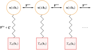
Figure 1. A schematic diagram of the heat-bath reinterpretation model of the stochastic fluid dynamics.
Download figure:
Standard image High-resolution imageIt is instructive to compare this model of the stochastic fluid dynamics with some other models of interacting many-body systems coupled to multiple baths, such as the harmonic lattice models [58, 59]. The Langevin equations for the harmonic lattice models and our model have a similar structure. Both types of dynamics have a reversible force that couples different lattice points together, and a dissipative force and a stochastic force related by the local FDT at each lattice point that is coupled to a heat bath [58, 59]. A major distinction is that the internal coupling in the harmonic lattice is linear and local (e.g., nearest-neighbor coupling), while that in the stochastic fluid dynamics is nonlinear and nonlocal, a difficulty inherent in fluid dynamics.
3. Potential landscape and flux field theory
We present the basics of the potential landscape and flux field theory, especially the nonequilibrium trinity, that will be used to develop and study the nonequilibrium thermodynamics of stochastic fluid systems in the context of the heat-bath reinterpretation. The results in this section are essentially contained in reference [52], but reformulated for the purpose of this article.
3.1. Fokker–Planck dynamics
The stochastic fluid dynamics in equation (4) is a Langevin equation for the set of state variables {u(k)}. The dynamics for the probability distribution of these state variables is governed by the corresponding Fokker–Planck equation [3, 4, 6, 52]

where Pt [u] = P[{u(k)}, t] is the transient probability distribution and ∇u(k) = ∂/∂u(k). For the diffusion matrix of the form in equation (8), equation (10) is the Edwards Fokker–Planck equation used in the study of homogeneous turbulence [6].
The Fokker–Planck equation can be written in the form of a continuity equation in the state space, ∂t Pt [u] = −∑k ∇u(k) ⋅ Jt (k)[u], where Jt (k)[u] = (Frev(k)[u] + Firr(k)[u])Pt [u] − Ds(k) ⋅ ∇u(−k) Pt [u] is the probability flux [3, 4, 43, 52]. The probability flux can be decomposed into a reversible part and an irreversible part according to their different time-reversal properties. The reversible probability flux, associated with the convective force, is identified as [3, 4, 43, 52]

while the irreversible probability flux, associated with both the viscous force and the stochastic force, is given by

Statistically steady states that do not vary with time are of interest. The steady-state probability distribution is denoted by Ps[u]. The steady-state probability fluxes, Js(k)[u], ![${\mathbf{J}}_{\mathrm{s}}^{\text{rev}}\left(\mathbf{k}\right)\left[\mathbf{u}\right]$](https://content.cld.iop.org/journals/1367-2630/22/11/113017/revision3/njpabc7d2ieqn2.gif) and
and ![${\mathbf{J}}_{\mathrm{s}}^{\text{irr}}\left(\mathbf{k}\right)\left[\mathbf{u}\right]$](https://content.cld.iop.org/journals/1367-2630/22/11/113017/revision3/njpabc7d2ieqn3.gif) , are defined with Pt
[u] replaced by Ps[u].
, are defined with Pt
[u] replaced by Ps[u].
3.2. Detailed balance breaking and nonequilibrium trinity
Steady states can be classified as equilibrium or nonequilibrium according to whether they preserve or break the time-reversal symmetry. Equilibrium steady states preserving the time-reversal symmetry obey detailed balance, which states that each elementary process is balanced by its time-reversed process. Nonequilibrium steady states that break detailed balance and time-reversal symmetry are of particular interest. For systems governed by the Fokker–Planck dynamics, detailed balance breaking in nonequilibrium steady states is signified by nonvanishing irreversible probability flux at the steady state [3], i.e.,  .
.
Both the probability distribution Ps and the irreversible probability flux  are needed to characterize nonequilibrium steady states. As a result of nonvanishing
  in nonequilibrium steady states, the irreversible force can be reformulated into a potential–flux form according to equation (12) (adapted to the steady state), leading to the nonequilibrium force decomposition [52]:

Here Φ[u] = − ln Ps[u] is the nonequilibrium potential landscape defined in terms of the steady-state probability distribution functional, and ![${\mathbf{V}}_{\mathrm{s}}^{\text{irr}}\left(\mathbf{k}\right)\left[\mathbf{u}\right]={\mathbf{J}}_{\mathrm{s}}^{\text{irr}}\left(\mathbf{k}\right)\left[\mathbf{u}\right]/{P}_{\mathrm{s}}\left[\mathbf{u}\right]$](https://content.cld.iop.org/journals/1367-2630/22/11/113017/revision3/njpabc7d2ieqn7.gif) is the steady-state irreversible probability flux velocity. Φ[u] is a (dimensionless) 'potential' in the state space rather than in the physical space or the wavevector space. (The term 'landscape' was inherited from the energy landscape theory.) Nonvanishing
is the steady-state irreversible probability flux velocity. Φ[u] is a (dimensionless) 'potential' in the state space rather than in the physical space or the wavevector space. (The term 'landscape' was inherited from the energy landscape theory.) Nonvanishing  is also an indicator of detailed balance breaking and time irreversibility just as
  is. Φ and
  can characterize nonequilibrium steady states as well as Ps and
  .
.
On the other hand, it can be verified that the irreversible force also has the following gradient form in the state space [52]:

where

 is the matrix inverse of Ds(k) in the transverse subspace. For Ds(k) in equation (8),
  . The quadratic form Φ0[u] is referred to as the Gaussian potential landscape, considering its relation to the Gaussian distribution
 ![${P}_{0}\left[\mathbf{u}\right]=\mathcal{N}\enspace {\mathrm{e}}^{-{{\Phi}}_{0}\left[\mathbf{u}\right]}$](https://content.cld.iop.org/journals/1367-2630/22/11/113017/revision3/njpabc7d2ieqn14.gif) , where
, where  is the normalization constant. Φ0 (or P0) is determined by the linear part of the stochastic fluid dynamics, namely, the viscous force Firr and the stochastic force characterized by Ds.
Equations (13) and (14) have distinct physical contents. The former connects Firr to nonequilibrium steady-state characterizations, Φ = − ln Ps and  , while the latter in terms of the Gaussian potential landscape Φ0 does not. However, as shown in the following, Φ0 (or P0) serves as a benchmark for Φ (or Ps).
Combining equations (13) and (14), we obtain the flux-deviation relation [52]

where Λ[u] = Φ0[u] − Φ[u] = ln(Ps[u]/P0[u]) (up to an additive constant) is the deviated potential landscape. It describes the deviation of the nonequilibrium potential landscape Φ (the steady-state distribution Ps) from the Gaussian potential landscape Φ0 (the Gaussian distribution P0). The flux-deviation relation reveals the connection between the steady-state irreversible probability flux velocity  and the deviation from the Gaussian feature Φ0 or P0. It shows that non-Gaussian statistics (Φ or Ps deviating from Φ0 or P0) is also a signature of detailed balance breaking and time-irreversibility in nonequilibrium steady states, equivalent to nonvanishing irreversible probability flux (
 or
or  ).
).
Moreover, by reformulating the steady-state Fokker–Planck equation in terms of the deviated potential landscape Λ, we obtain the following nonequilibrium source equation [52]:
where

We observe some general features of this equation. The three terms on the lhs of this equation all contain the deviated potential landscape Λ[u], a nonequilibrium signature of the steady state when it is non-constant. The rhs of this equation B[u] is referred to as the detailed balance breaking functional. Nonvanishing B[u] acts as a source term in equation (17), generating a non-constant Λ[u] (otherwise B[u] vanishes), which signifies the nonequilibrium nature of the steady state. This perspective shows that B[u] ≠ 0 is a more fundamental characterization of detailed balance breaking. The expression of B[u] in equation (18) suggests that detailed balance breaking (B[u] ≠ 0) represents the mechanical imbalance in the driving forces of the stochastic fluid dynamics, namely, the reversible convective force Frev, the irreversible viscous force Firr, and the stochastic force characterized by Ds. Equation (17) can also be reformulated in terms of  using the flux-deviation relation. Hence, B[u] is also the source of
  .
.
The nonequilibrium source equation, equation (17), and the flux-deviation relation, equation (16), together establish what we call the nonequilibrium trinity, schematically shown in figure 2. The nonequilibrium trinity is a unified entity consisting of three interrelated elements, which characterizes the nonequilibrium irreversible nature of the fluid system. The three elements are detailed balance breaking, non-Gaussian potential landscape and irreversible probability flux. The latter two elements are connected by the flux-deviation relation, both serving as signatures of detailed balance breaking and time irreversibility in nonequilibrium steady states in fluid systems. The nonequilibrium source equation demonstrates that this pair of elements is generated by detailed balance breaking that represents the mechanical imbalance in the driving forces of the stochastic fluid dynamics. A systematic investigation of the nonequilibrium trinity in relation to the nonequilibrium fluid dynamics, the turbulence energy cascade, and the four-fifth law in fully developed turbulence can be found in reference [52], which will not be discussed here.

Figure 2. A schematic representation of the nonequilibrium trinity.
Download figure:
Standard image High-resolution image4. Nonequilibrium thermodynamics of stochastic fluid systems
We investigate the nonequilibrium thermodynamics of stochastic fluid systems in the context of the heat-bath reinterpretation using the potential landscape and flux field theory. We first develop the set of nonequilibrium thermodynamic equations and summarize the results. Then we focus on the steady-state nonequilibrium thermodynamics. We further investigate the origin of detailed balance breaking and the connection of nonequilibrium thermodynamics to the nonequilibrium trinity construct.
4.1. Energy balance equation
The Hamiltonian (kinetic energy) of the velocity field is H[u] = (1/2)∫u2(x)dx = (L3/2)∑k
u(−k) ⋅ u(k). The energy contained in mode k is identified as E(k) = (L3/2)u(−k) ⋅ u(k). (Thermodynamic quantities are divided equally between k and −k that were previously associated with one mode.) Its ensemble average gives the average energy in mode k: ![$\mathcal{E}\left(\mathbf{k},t\right)={\langle E\left(\mathbf{k}\right)\rangle }_{t}=\int E\left(\mathbf{k}\right){P}_{t}\left[\mathbf{u}\right]\delta \mathbf{u}$](https://content.cld.iop.org/journals/1367-2630/22/11/113017/revision3/njpabc7d2ieqn22.gif) , where Pt
[u] obeys the Fokker–Planck equation and ∫δ
u represents integration in the state space. The total average energy
, where Pt
[u] obeys the Fokker–Planck equation and ∫δ
u represents integration in the state space. The total average energy ![$\mathcal{E}\left(t\right)={\langle H\left[\mathbf{u}\right]\rangle }_{t}$](https://content.cld.iop.org/journals/1367-2630/22/11/113017/revision3/njpabc7d2ieqn23.gif) is the internal energy of the system in the context of the heat-bath reinterpretation.
is the internal energy of the system in the context of the heat-bath reinterpretation.
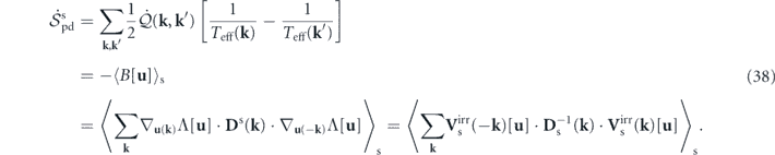
Using the Fokker–Planck equation, the energy balance equation at mode k is found to be [6, 8, 16, 29, 52]

where ![$\mathcal{T}\left(\mathbf{k},t\right)=\mathcal{R}\left\{{L}^{3}\left[-\mathrm{i}\mathbf{k}\cdot {\sum }_{{\mathbf{k}}^{\prime }}{\langle \mathbf{u}\left(\mathbf{k}-{\mathbf{k}}^{\prime }\right)\mathbf{u}\left({\mathbf{k}}^{\prime }\right)\cdot \mathbf{u}\left(-\mathbf{k}\right)\rangle }_{t}\right]\right\}$](https://content.cld.iop.org/journals/1367-2630/22/11/113017/revision3/njpabc7d2ieqn24.gif) is the energy transfer rate associated with the convective force,
is the energy transfer rate associated with the convective force,  is the energy dissipation rate associated with the viscous force, and
  is the energy injection rate associated with the stochastic force.
  denotes taking the real part.
In the context of the heat-bath reinterpretation, the energy dissipation and the energy injection at each mode, associated with the viscous force and the stochastic force at that mode, both originate from the interactions between the mode and the associated heat bath. Hence, these two parts can be combined together and reinterpreted as the heat flow rate from mode k to the heat bath. That is, ![$\dot {\mathcal{Q}}\left(\mathbf{k},t\right)=\mathcal{D}\left(\mathbf{k},t\right)-\mathcal{I}\left(\mathbf{k},t\right)=-\mathcal{R}\left\{{\langle {\mathbf{V}}_{t}^{\text{irr}}\left(\mathbf{k}\right)\left[\mathbf{u}\right]\cdot {\nabla }_{\mathbf{u}\left(\mathbf{k}\right)}H\left[\mathbf{u}\right]\rangle }_{t}\right\}$](https://content.cld.iop.org/journals/1367-2630/22/11/113017/revision3/njpabc7d2ieqn28.gif) , where the last expression with
, where the last expression with  can be verified using the Fokker–Planck equation. The total heat flow rate from the system to all the heat baths is then
 ![$\dot {\mathcal{Q}}\left(t\right)=-{\langle {\sum }_{\mathbf{k}}{\mathbf{V}}_{t}^{\text{irr}}\left(\mathbf{k}\right)\left[\mathbf{u}\right]\cdot {\nabla }_{\mathbf{u}\left(\mathbf{k}\right)}H\left[\mathbf{u}\right]\rangle }_{t}$](https://content.cld.iop.org/journals/1367-2630/22/11/113017/revision3/njpabc7d2ieqn30.gif) . The energy balance equation at mode k in equation (19) can now be rewritten as
. The energy balance equation at mode k in equation (19) can now be rewritten as

Summing over k, we obtain the total energy balance equation

where we have used the property  associated with the conservative nature of the convective force.
Equations (20) and (21) represent the first law of thermodynamics. Equation (20) shows that the change of the internal energy at mode k is due to the redistribution of energy among different modes by the reversible convective force and the transfer of heat between the mode and the associated heat bath. On the overall level, equation (21) states that the change of the total internal energy of the system is due to the transfer of heat between the system and all the heat baths. This is a manifestation of energy conservation when there is no work-related energy input or output (e.g., through time-dependent parameters).
4.2. Gaussian cross entropy balance equation
Insights can be gained by studying the balance equation associated with the Gaussian potential landscape Φ0[u]. Combining equations (8), (9) and (15), we find Φ0[u] = ∑k
E(k)/Teff(k), where E(k) is the energy at mode k and Teff(k) is the effective temperature. The expression of Φ0 at mode k is identified as Φ0(k) = E(k)/Teff(k). Its ensemble average is defined as the Gaussian cross entropy at mode k:  . The total Gaussian cross entropy is given by
 ![$\mathcal{G}\left(t\right)={\langle {{\Phi}}_{0}\left[\mathbf{u}\right]\rangle }_{t}=-\int {P}_{t}\left[\mathbf{u}\right]\mathrm{ln}\enspace {P}_{0}\left[\mathbf{u}\right]\delta \mathbf{u}$](https://content.cld.iop.org/journals/1367-2630/22/11/113017/revision3/njpabc7d2ieqn33.gif) , which shows that
, which shows that  is the cross entropy between the Gaussian distribution P0[u] and the transient distribution Pt
[u].
is the cross entropy between the Gaussian distribution P0[u] and the transient distribution Pt
[u].
From the expression  and the energy balance equation in equation (20), we find

The last term is the entropy flow rate at mode k: ![${\dot {\mathcal{S}}}_{\mathrm{fl}}\left(\mathbf{k},t\right)=\dot {\mathcal{Q}}\left(\mathbf{k},t\right)/{T}_{\text{eff}}\left(\mathbf{k}\right)=\mathcal{R}\left\{{\langle {\mathbf{V}}_{t}^{\text{irr}}\left(-\mathbf{k}\right)\left[\mathbf{u}\right]\cdot {\mathbf{D}}_{\mathrm{s}}^{-1}\left(\mathbf{k}\right)\cdot {\mathbf{F}}^{\text{irr}}\left(\mathbf{k}\right)\left[\mathbf{u}\right]\rangle }_{t}\right\}$](https://content.cld.iop.org/journals/1367-2630/22/11/113017/revision3/njpabc7d2ieqn36.gif) , where the last step can be verified using the expression of
, where the last step can be verified using the expression of  . The first term on the rhs of equation (22), with a negative sign, is the average detailed balance breaking at mode k:
 ![$\mathcal{B}\left(\mathbf{k},t\right)=-\mathcal{T}\left(\mathbf{k},t\right)/{T}_{\text{eff}}\left(\mathbf{k}\right)=\mathcal{R}\left\{{\langle {\mathbf{F}}^{\text{rev}}\left(-\mathbf{k}\right)\left[\mathbf{u}\right]\cdot {\mathbf{D}}_{\mathrm{s}}^{-1}\left(\mathbf{k}\right)\cdot {\mathbf{F}}^{\text{irr}}\left(\mathbf{k}\right)\left[\mathbf{u}\right]\rangle }_{t}\right\}$](https://content.cld.iop.org/journals/1367-2630/22/11/113017/revision3/njpabc7d2ieqn38.gif) , where the last step can be verified using the expression of
, where the last step can be verified using the expression of  .
.  is the ensemble average of
 ![$B\left(\mathbf{k}\right)\left[\mathbf{u}\right]=\mathcal{R}\left\{{\mathbf{F}}^{\text{rev}}\left(-\mathbf{k}\right)\left[\mathbf{u}\right]\cdot {\mathbf{D}}_{\mathrm{s}}^{-1}\left(\mathbf{k}\right)\cdot {\mathbf{F}}^{\text{irr}}\left(\mathbf{k}\right)\left[\mathbf{u}\right]\right\}$](https://content.cld.iop.org/journals/1367-2630/22/11/113017/revision3/njpabc7d2ieqn41.gif) , which is the mode-wise expression of the detailed balance breaking functional B[u] in equation (18).
, which is the mode-wise expression of the detailed balance breaking functional B[u] in equation (18).
Thus the balance equation for the Gaussian cross entropy at mode k has the form

Summing over k, we obtain the total Gaussian cross entropy balance equation

where the total (average) detailed balance breaking is given by ![$\mathcal{B}\left(t\right)={\langle B\left[\mathbf{u}\right]\rangle }_{t}=-{\sum }_{\mathbf{k}}\mathcal{T}\left(\mathbf{k},t\right)/{T}_{\text{eff}}\left(\mathbf{k}\right)$](https://content.cld.iop.org/journals/1367-2630/22/11/113017/revision3/njpabc7d2ieqn42.gif) , and the total entropy flow rate has the expression
, and the total entropy flow rate has the expression ![${\dot {\mathcal{S}}}_{\mathrm{fl}}\left(t\right)={\sum }_{\mathbf{k}}\dot {\mathcal{Q}}\left(\mathbf{k},t\right)/{T}_{\text{eff}}\left(\mathbf{k}\right)={\langle {\sum }_{\mathbf{k}}{\mathbf{V}}_{t}^{\text{irr}}\left(-\mathbf{k}\right)\left[\mathbf{u}\right]\cdot {\mathbf{D}}_{\mathrm{s}}^{-1}\left(\mathbf{k}\right)\cdot {\mathbf{F}}^{\text{irr}}\left(\mathbf{k}\right)\left[\mathbf{u}\right]\rangle }_{t}$](https://content.cld.iop.org/journals/1367-2630/22/11/113017/revision3/njpabc7d2ieqn43.gif) .
.
The Gaussian cross entropy balance equation at mode k in equation (23) is mathematically equivalent to the energy balance equation at mode k in equation (20), as the former is obtained from the latter by dividing it with Teff(k). Hence, it is connected to the first law of thermodynamics. On the other hand, the total Gaussian cross entropy balance equation reveals the connection among Gaussian cross entropy, detailed balance breaking and entropy flow, especially the connection between the latter two at the steady state. This also allows it to make connection with the second law of thermodynamics represented by the next thermodynamic equation.
4.3. Nonequilibrium entropy balance equation
We define the nonequilibrium entropy of the system as the Gibbs–Boltzmann entropy of the transient probability distribution Pt
[u], namely, ![$\mathcal{S}\left(t\right)={\langle S\left[\mathbf{u}\right]\rangle }_{t}=-\int {P}_{t}\left[\mathbf{u}\right]\mathrm{ln}\enspace {P}_{t}\left[\mathbf{u}\right]\delta \mathbf{u}$](https://content.cld.iop.org/journals/1367-2630/22/11/113017/revision3/njpabc7d2ieqn44.gif) , where S[u] = − ln Pt
[u]. In general,
, where S[u] = − ln Pt
[u]. In general,  does not have the explicit mode-sum form to be defined at each mode, in contrast with
  and
and  . In addition,
  is the entropy associated with the hydrodynamic modes [29], which is different from the entropy associated with the molecular degrees of freedom [30, 31].
Using the Fokker–Planck equation, the rate of change of  is found to be
 ![$\dot {\mathcal{S}}\left(t\right)={\langle {\sum }_{\mathbf{k}}{\mathbf{V}}_{t}^{\text{irr}}\left(\mathbf{k}\right)\left[\mathbf{u}\right]\cdot {\nabla }_{\mathbf{u}\left(\mathbf{k}\right)}S\left[\mathbf{u}\right]\rangle }_{t}$](https://content.cld.iop.org/journals/1367-2630/22/11/113017/revision3/njpabc7d2ieqn50.gif) , where we have used ∑k
∇u(k) ⋅ Frev(k)[u] = 0 [52]. Furthermore, from equation (12), we obtain
, where we have used ∑k
∇u(k) ⋅ Frev(k)[u] = 0 [52]. Furthermore, from equation (12), we obtain ![${\nabla }_{\mathbf{u}\left(-\mathbf{k}\right)}S\left[\mathbf{u}\right]={\mathbf{D}}_{\mathrm{s}}^{-1}\left(\mathbf{k}\right)\cdot {\mathbf{V}}_{t}^{\text{irr}}\left(\mathbf{k}\right)\left[\mathbf{u}\right]-{\mathbf{D}}_{\mathrm{s}}^{-1}\left(\mathbf{k}\right)\cdot {\mathbf{F}}^{\text{irr}}\left(\mathbf{k}\right)\left[\mathbf{u}\right]$](https://content.cld.iop.org/journals/1367-2630/22/11/113017/revision3/njpabc7d2ieqn51.gif) . Inserting it into the expression of
. Inserting it into the expression of  , we get the nonequilibrium entropy balance equation

where ![${\dot {\mathcal{S}}}_{\mathrm{fl}}\left(t\right)={\langle {\sum }_{\mathbf{k}}{\mathbf{V}}_{t}^{\text{irr}}\left(-\mathbf{k}\right)\left[\mathbf{u}\right]\cdot {\mathbf{D}}_{\mathrm{s}}^{-1}\left(\mathbf{k}\right)\cdot {\mathbf{F}}^{\text{irr}}\left(\mathbf{k}\right)\left[\mathbf{u}\right]\rangle }_{t}$](https://content.cld.iop.org/journals/1367-2630/22/11/113017/revision3/njpabc7d2ieqn53.gif) is the total entropy flow rate from the system to the heat baths defined previously. Hence,
is the total entropy flow rate from the system to the heat baths defined previously. Hence, ![${\dot {\mathcal{S}}}_{\mathrm{p}\mathrm{d}}\left(t\right)={\langle {\sum }_{\mathbf{k}}{\mathbf{V}}_{t}^{\text{irr}}\left(-\mathbf{k}\right)\left[\mathbf{u}\right]\cdot {\mathbf{D}}_{\mathrm{s}}^{-1}\left(\mathbf{k}\right)\cdot {\mathbf{V}}_{t}^{\text{irr}}\left(\mathbf{k}\right)\left[\mathbf{u}\right]\rangle }_{t}$](https://content.cld.iop.org/journals/1367-2630/22/11/113017/revision3/njpabc7d2ieqn54.gif) can be identified as the total entropy production rate.
can be identified as the total entropy production rate.
The total entropy production rate  is nonnegative, since it is the ensemble average of a positive-definite quadratic form of
 ![${\mathbf{V}}_{t}^{\text{irr}}\left[\mathbf{u}\right]$](https://content.cld.iop.org/journals/1367-2630/22/11/113017/revision3/njpabc7d2ieqn56.gif) in the state space. This implies
in the state space. This implies  . That is, the total entropy of the system plus the baths does not decrease with time, a statement of the second law of thermodynamics.
4.4. Summary of the nonequilibrium thermodynamics
The nonequilibrium thermodynamics for stochastic fluid systems in the context of the heat-bath reinterpretation is summarized in the following. The nonequilibrium thermodynamic equations on the overall level read

and we also have two equations at each mode

In these equations,  is the internal energy (of the hydrodynamic modes);
  is the Gaussian cross entropy;
  is the nonequilibrium entropy;
  is the detailed balance breaking;
  is the heat flow rate;
  is the entropy flow rate; and
  is the entropy production rate. Their expressions are listed below for completeness:


Their mode-wise expressions can be obtained by exploiting the mode-sum form and taking the real part. The nonequilibrium thermodynamic equations and thermodynamic quantities have also been reformulated in the physical space in appendix
The energy balance equation,  , represents energy conservation and the first law of thermodynamics. The nonequilibrium entropy balance equation,
  , with nonnegative entropy production, represents the second law of thermodynamics. The Gaussian cross entropy balance equation,
  , relates the first and second laws of thermodynamics. The mathematical equivalence of the two equations in equation (27) demonstrates its connection to the first law of thermodynamics, while the relation it reveals between detailed balance breaking and entropy flow is connected to the second law of thermodynamics.
4.5. Steady-state nonequilibrium thermodynamics
The nonequilibrium thermodynamics at the steady state is of particular interest. At the steady state  ,
,  and
and  (also
(also  and
and  ) become time-independent, as the transient distribution Pt
[u] is replaced by the steady-state distribution Ps[u]. As a result, the set of nonequilibrium thermodynamic equations on the overall level, equation (26), reduces to
) become time-independent, as the transient distribution Pt
[u] is replaced by the steady-state distribution Ps[u]. As a result, the set of nonequilibrium thermodynamic equations on the overall level, equation (26), reduces to

and at each mode we have

which is mathematically equivalent to the other mode-wise equation  . The subscript or superscript s indicates the steady state. All other thermodynamic quantities in equations (26) and (27) vanish. Also note that
  .
.
We discuss the implications of the steady-state nonequilibrium thermodynamics. Equation (35) reveals the connection of detailed balance breaking to entropy flow and entropy production at the steady state, thanks to the Gaussian cross entropy balance equation. For nonequilibrium steady states violating detailed balance, the average detailed balance breaking  is nonzero in general. Accordingly, there is nonzero entropy production and entropy flow at nonequilibrium steady states. The nonnegativity of entropy production then indicates that
  , which means there is net entropy flow from the system to the heat baths, transferring out the entropy produced within the system to maintain a constant system entropy at the steady state. Entropy flow is carried by heat flow, as reflected in the expression
  . This implies that heat flows at some modes do not vanish. The same goes for energy transfer according to equation (36). In other words, there are heat flows between the system and the heat baths, accompanied by energy flows within the system between different modes. Some heat baths act as energy sources while some as energy sinks, so that the total heat flow
  remains zero at the steady state due to conservation of energy. Nonzero entropy production and entropy flow accompanied by steady energy flow and heat flow are thermodynamic signatures of nonequilibrium steady states that break detailed balance and time-reversal symmetry. The relations revealed in the steady-state nonequilibrium thermodynamics are further investigated in its origin and in relation to the nonequilibrium trinity in the following.
4.6. Origin of detailed balance breaking
Previously, we interpreted detailed balance breaking as a form of mechanical imbalance in the driving forces of the stochastic fluid dynamics, based on the expression of B[u] in equation (18). In the context of the heat-bath reinterpretation of the stochastic fluid dynamics, however, it is intuitive that nonequilibrium steady states with detailed balance breaking are sustained by the temperature differences of the heat baths (thermal imbalance). To reveal the connection between detailed balance breaking and temperature nonuniformity, we notice that, after some algebra, the expression of B[u] in equation (18) can be reformulated as

where ![$T\left(\mathbf{k},{\mathbf{k}}^{\prime }\right)\left[\mathbf{u}\right]=-{L}^{3}\mathcal{R}\left\{\left(\mathrm{i}/2\right)\left(\mathbf{k}+{\mathbf{k}}^{\prime }\right)\cdot \mathbf{u}\left(\mathbf{k}-{\mathbf{k}}^{\prime }\right)\mathbf{u}\left({\mathbf{k}}^{\prime }\right)\cdot \mathbf{u}\left(-\mathbf{k}\right)\right\}$](https://content.cld.iop.org/journals/1367-2630/22/11/113017/revision3/njpabc7d2ieqn79.gif) . Here T(k, k')[u] satisfies T(k', k)[u] = −T(k, k')[u] and can be interpreted as the energy transfer rate from k' to k for a velocity field u [8, 29, 60]. (A cautionary remark: T(k, k')[u] involves three modes instead of two.) It is related to the energy transfer rate at mode k by
. Here T(k, k')[u] satisfies T(k', k)[u] = −T(k, k')[u] and can be interpreted as the energy transfer rate from k' to k for a velocity field u [8, 29, 60]. (A cautionary remark: T(k, k')[u] involves three modes instead of two.) It is related to the energy transfer rate at mode k by ![$\mathcal{T}\left(\mathbf{k},t\right)={\sum }_{{\mathbf{k}}^{\prime }}{\langle T\left(\mathbf{k},{\mathbf{k}}^{\prime }\right)\left[\mathbf{u}\right]\rangle }_{t}$](https://content.cld.iop.org/journals/1367-2630/22/11/113017/revision3/njpabc7d2ieqn80.gif) .
.
According to the above expression of B[u], when all the heat baths have the same temperature, i.e., Teff(k) = Teff, the detailed balance breaking functional B[u] vanishes for all velocity fields in the state space. This means the fluid system preserves detailed balance and has an equilibrium steady state. Indeed, the stochastic fluid dynamics in this case describes a fluid with a global equilibrium temperature Teff, which we studied in detail in reference [52]. Interestingly, the reverse is also true. We have the following theorem, proven in appendix
Theorem. The necessary and sufficient condition for detailed balance, namely B[u] = 0 for all velocity fields in the state space, is that the effective temperature distribution Teff(k) (k ≠ 0) is uniform.
This theorem immediately implies that temperature difference of the heat baths is the necessary and sufficient condition for detailed balance breaking. From the perspective of the heat-bath reinterpretation, it is natural to view the temperature nonuniformity of the heat baths as the physical origin of detailed balance breaking, instead of the other way around.
4.7. Nonequilibrium thermodynamics in relation to nonequilibrium trinity
To develop a more coherent picture of the origin, characteristics and manifestations of the nonequilibrium nature of stochastic fluid systems, we synthesize the steady-state nonequilibrium thermodynamics, the nonequilibrium trinity construct, and the origin of detailed balance breaking. In particular, by combining equations (35), (37), (34), and (16), we find that the steady-state entropy production, a crucial thermodynamic property of nonequilibrium steady states, has the following expressions:
These four different expressions are in terms of the temperature difference, the detailed balance breaking, the deviated potential landscape, and the irreversible probability flux, respectively. The first element is the origin of detailed balance breaking, while the last three elements form the nonequilibrium trinity construct.
In the first expression, ![$\dot {\mathcal{Q}}\left(\mathbf{k},{\mathbf{k}}^{\prime }\right)\equiv \mathcal{T}\left(\mathbf{k},{\mathbf{k}}^{\prime }\right)={\langle T\left(\mathbf{k},{\mathbf{k}}^{\prime }\right)\left[\mathbf{u}\right]\rangle }_{\mathrm{s}}$](https://content.cld.iop.org/journals/1367-2630/22/11/113017/revision3/njpabc7d2ieqn81.gif) .
.  is the energy transfer rate from k' to k at the steady state. Given the steady-state energy balance equation
  , the energy flow within the system conducted by the reversible convective force can be interpreted as the heat flow through the system driven by the temperature differences of the heat baths. Hence, we reinterpret
  as the heat flow rate from k' to k and denote it by
  . This first expression of entropy production has the form of paired thermodynamic fluxes (heat flux) and thermodynamic forces (inverse temperature difference). However, the flux–force relationship can be highly nonlinear if the system is far from equilibrium (e.g., turbulence).
The last three expressions indicate that the steady-state entropy production rate is a quantitative measure of detailed balance breaking, non-Gaussian statistics and time irreversibility in nonequilibrium steady states. That it quantifies detailed balance breaking is evident in the expression ![${\dot {\mathcal{S}}}_{\mathrm{p}\mathrm{d}}^{\mathrm{s}}=-{\langle B\left[\mathbf{u}\right]\rangle }_{\mathrm{s}}$](https://content.cld.iop.org/journals/1367-2630/22/11/113017/revision3/njpabc7d2ieqn86.gif) . The last two expressions are positive-definite quadratic forms of ∇u
Λ [u] and
. The last two expressions are positive-definite quadratic forms of ∇u
Λ [u] and ![${\mathbf{V}}_{\mathrm{s}}^{\text{irr}}\left[\mathbf{u}\right]$](https://content.cld.iop.org/journals/1367-2630/22/11/113017/revision3/njpabc7d2ieqn87.gif) , where Ds and
, where Ds and  may be regarded as metric matrices in the state space. This means
  also measures the squared magnitude of ∇u
Λ [u] (non-Gaussian statistics) and
also measures the squared magnitude of ∇u
Λ [u] (non-Gaussian statistics) and ![${\mathbf{V}}_{\mathrm{s}}^{\text{irr}}\left[\mathbf{u}\right]$](https://content.cld.iop.org/journals/1367-2630/22/11/113017/revision3/njpabc7d2ieqn90.gif) (time irreversibility) in nonequilibrium steady states.
(time irreversibility) in nonequilibrium steady states.
The four expressions have different levels of 'fundamentalness'. The last three expressions demonstrate that the steady-state entropy production is a manifestation of the nonequilibrium trinity. In these three expressions, the one in terms of detailed balance breaking is more fundamental than the other two, from the perspective that detailed balance breaking is the source of the non-Gaussian potential landscape and the irreversible probability flux, according to the nonequilibrium source equation in equation (17). The last two expressions are equivalent to each other according to the flux-deviation relation in equation (16), which places the non-Gaussian potential landscape and the irreversible probability flux on an equal footing. Moreover, the first expression in terms of the temperature difference is the most fundamental, since the origin of detailed balance breaking has been traced to the temperature difference. Hence, in the context of the heat-bath reinterpretation, the temperature nonuniformity of the heat baths is the physical origin of detailed balance breaking that generates the non-Gaussian potential landscape and the irreversible probability flux on the dynamical level, which in turn is manifested on the thermodynamical level as the steady-state entropy production accompanied by energy flow, heat flow and entropy flow. A schematic diagram of the above logic is shown in figure 3.
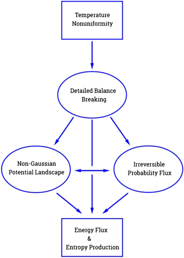
Figure 3. A schematic representation of the causal connections of the effective temperature nonuniformity, the nonequilibrium trinity construct, and the steady-state nonequilibrium thermodynamics.
Download figure:
Standard image High-resolution image5. Nonequilibrium thermodynamics of turbulence
In this section we investigate what insights can be gained on turbulence by presenting a nonequilibrium thermodynamic perspective of turbulence and studying its nonequilibrium thermodynamics in the context of the heat-bath reinterpretation. We first discuss a quantitative measure of the effective temperature nonuniformity, and reveal its connection to the Reynolds number, a high value of which signifies turbulence. Then we present the nonequilibrium thermodynamic perspective of turbulence energy cascade and study the corresponding nonequilibrium thermodynamics.
5.1. Measures of effective temperature nonuniformity
The temperature difference of the heat baths as the origin of detailed balance breaking plays a critical role in the nonequilibrium dynamics and thermodynamics of stochastic fluid systems. A quantitative measure of temperature nonuniformity will provide an overall characterization of the degree of departure from thermodynamic equilibrium. We investigate such measures.
The effective temperature was defined as Teff(k) = W(k)L3/(2νk2), where W(k) > 0 (k ≠ 0) is the energy injection rate per unit mass. We assume that the total energy injection rate per unit mass is finite, i.e., ∑k
W(k) = ɛ, (0 < ɛ < ∞). Here ɛ is also the total energy dissipation rate per unit mass at the steady state, according to the steady-state energy balance equation. This assumption implies that  , where kL
= 2π/L is the smallest nonzero wavenumber. The upper bound is referred to as the maximum temperature nonuniformity (explained later) and denoted as
, where kL
= 2π/L is the smallest nonzero wavenumber. The upper bound is referred to as the maximum temperature nonuniformity (explained later) and denoted as

The average effective temperature  is formally defined as the arithmetic mean of all the effective temperatures. Then
  further implies that
  is (almost) zero, i.e.,
  , since there are many wavevectors (although not infinitely many from a physical perspective, for the continuum description of the fluid to be valid).
The overall difference between the effective temperature distribution and the average effective temperature is a reasonable measure of the temperature nonuniformity. A class of such measures can be constructed based on the p-norm:  , for p ∈ [1, ∞]. By making another moderate assumption,
  , (0 < α ⩽ 1 ⩽ β < ∞), it can be shown that these p-norm measures are equivalent to the measure
  in the sense that

where  and
and  . This relation also justifies
  as the 'maximum temperature nonuniformity'. When energy injection is concentrated at the large spatial scale close to the system size L, as for the 3D turbulence case, Cp
is close to one and thus all these p-norm measures are close to
as the 'maximum temperature nonuniformity'. When energy injection is concentrated at the large spatial scale close to the system size L, as for the 3D turbulence case, Cp
is close to one and thus all these p-norm measures are close to  . When energy injection is less concentrated at the large spatial scale, ||ΔTeff||p
deviates from (is less than)
. When energy injection is less concentrated at the large spatial scale, ||ΔTeff||p
deviates from (is less than)  , but the deviation is bounded by the numerical factor Cp
. Therefore, we may use
, but the deviation is bounded by the numerical factor Cp
. Therefore, we may use  as the common measure of the temperature nonuniformity of the heat baths.
5.2. Connection of effective temperature nonuniformity to Reynolds number
The effective temperature nonuniformity  measures the degree of departure from thermodynamic equilibrium. On the other hand, the Reynolds number Re in fluid dynamics, whose values indicate different flow patterns (laminar or turbulent), is also related to the notion of 'distance' from equilibrium. We show that they are actually connected.
A basic distinction between Re and  is that the former is dimensionless, while the latter is not. The Reynolds number is defined as the ratio between the nonlinear convective force and the viscous force. On the other hand, the effective temperature is defined by the viscous force and the stochastic force through the FDT. To bridge the gap in dimensions, we use the steady-state energy balance equation (see equation (19) and (36)),
  , which maps forces to rates of energy change. We introduce a dimensionless quantity related to the effective temperature at each mode,
  , which is termed the injection-dissipation number, as it characterizes the relative intensity between energy injection (stochastic force) and energy dissipation (viscous force). We can also introduce the Reynolds number at each mode, which characterizes the relative intensity between energy transfer (nonlinear convective force) and energy dissipation (viscous force), as follows:
  , where
  and
and  . In the steady-state setting, these two dimensionless quantities are related by Re(k) = |ID
(k) − 1|.
. In the steady-state setting, these two dimensionless quantities are related by Re(k) = |ID
(k) − 1|.
The Reynolds number that indicates different flow patterns is the one at the large spatial scale, where energy injection concentrates ( ) and energy dissipation is negligible (
 ). Energy balance then indicates
  . Combined with the estimate
  suggested by the structure of
  , it follows that u(kL
) ∼ (ɛL)1/3. Hence, Re(kL
) ∼ u(kL
)/(kL
ν) ∼ ɛ1/3
L4/3/ν, which also has the well-known form
, it follows that u(kL
) ∼ (ɛL)1/3. Hence, Re(kL
) ∼ u(kL
)/(kL
ν) ∼ ɛ1/3
L4/3/ν, which also has the well-known form  , where
  is the Kolmogorov length scale [16]. On the other hand, combining the estimates
 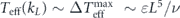 and
and  , we have
  . Therefore, Re(kL
) ∼ ID
(kL
), as expected from the relation Re(k) = |ID
(k) − 1| and ID
(kL
) ≫ 1 as energy injection dominates energy dissipation. In summary, we have obtained
. Therefore, Re(kL
) ∼ ID
(kL
), as expected from the relation Re(k) = |ID
(k) − 1| and ID
(kL
) ≫ 1 as energy injection dominates energy dissipation. In summary, we have obtained

The above relations have established a connection between Reynolds number and effective temperature nonuniformity. Re(kL
) and  are both positively correlated with ɛ and L and negatively correlated with ν. High Reynolds number indicating turbulent flows in the far-from-equilibrium regime corresponds to strong nonuniformity in the heat bath temperatures.
5.3. Nonequilibrium thermodynamic perspective and thermodynamics of turbulence
Turbulent fluid dynamics in the far-from-equilibrium regime with high Reynolds numbers can also be viewed from the perspective of nonequilibrium thermodynamics driven by highly nonuniform effective temperatures in the context of the heat-bath reinterpretation. The thermodynamic viewpoint may be more intuitive in certain aspects. In the following we present the nonequilibrium thermodynamic perspective of turbulence and study its nonequilibrium thermodynamics.
Energy cascade is arguably the most important physical picture of turbulence. In the direct energy cascade picture, energy is transferred by nonlinear convection from the large scales of motion to the small scales, where it is dissipated by molecular viscosity. The directional energy flow across scales in energy cascade is a signature of the nonequilibrium irreversible nature of turbulence. In the context of the heat-bath reinterpretation, we show that turbulence energy cascade has the intuitive interpretation of heat conduction in the wavevector space. In particular, the energy flux across scales in energy cascade has the natural interpretation of the heat flux through the wavenumber dimension, which is conducted by the nonlinear convective force and driven by the temperature difference of the heat baths at the large and small scales. The nonequilibrium irreversibility of turbulence energy cascade can be quantified by the steady-state entropy production in the heat conduction process in the wavenumber dimension. A schematic of the nonequilibrium thermodynamic perspective of turbulence energy cascade is shown in figure 4.

Figure 4. A schematic diagram of turbulence energy cascade interpreted as heat conduction in the wavenumber dimension.
Download figure:
Standard image High-resolution image
5.3.1. Cumulative energy balance equation
To substantiate the above nonequilibrium thermodynamic picture of turbulence, some preparations are needed. We first consider the cumulative energy balance equation at the steady state [16]. The cumulative energy of the modes up to wavenumber κ is defined as 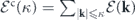 . Similarly, the cumulative energy dissipation rate is given by
  , and the cumulative energy injection rate reads
  . To agree with convention, the cumulative energy transfer rate (also referred to as the cumulative energy flux) is defined with an additional negative sign, namely
 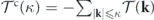 , which represents the rate of energy transfer out of the modes |k| ⩽ κ. In terms of the cumulative quantities, the steady-state energy balance equation
  becomes

In the context of the heat-bath reinterpretation, energy injection and energy dissipation both originate from the interactions of the modes with the heat baths. Hence, they were combined to define the heat flow rate  from mode k to the heat bath. Accordingly, we define the cumulative heat flow rate as
  . The steady-state cumulative energy balance equation can now be rewritten as

which means at the steady state the rate of energy transfer out of the modes |k| ⩽ κ by the nonlinear convective force is equal to the rate of heat flow into these modes from the heat baths. This is a manifestation of energy conservation at the steady state representing the first law of thermodynamics. Later we shall apply it to the turbulence energy cascade process.
5.3.2. Assumptions for the existence of an inertial subrange
Under certain assumptions there exists an inertial subrange of energy cascade in fully developed turbulence, throughout which the cumulative energy flux  is (approximately) constant [16]. In the setting of the steady-state forced turbulence described by the stochastic NSE, these assumptions can be summarized as follows [16, 52]: (1) the stochastic force acts mainly at the large scale comparable to the system size L; (2) the steady state of the system has a finite mean energy per unit mass in the limit ν → 0; (3) the stochastic force does not depend on the viscosity ν.
The first assumption represents large-scale forcing, which means energy injection is concentrated at the large spatial scales (small wavenumbers). This requires the significant values of W(k) to be contained in a range (0, kI ] with the characteristic wavenumber kL = 2π/L, beyond which W(k) decreases rapidly with k. The third assumption requires W(k) to be independent of ν. In particular, the total energy injection rate per unit mass ∑k W(k) = ɛ, which is also equal to the total energy dissipation rate per unit mass at the steady state, does not depend on ν. These two assumptions can be fulfilled by suitable forms of W(k).
The second assumption can be formulated as  . There is no freedom to control whether this assumption can be fulfilled or not. But if it is indeed fulfilled, then for any finite wavenumber κ, it follows that [16]:
  (ν → 0). Since at the steady state the total energy dissipation rate per unit mass remains a nonzero constant ɛ (determined by the energy injection rate that is independent of ν), this means energy dissipation is concentrated at k = ∞ in the limit ν → 0 (Re → ∞). For a small but finite ν, energy dissipation is concentrated at the large wavenumbers (small spatial scales), with the characteristic wavenumber kη
= 2π/η, where η is the Kolmogorov length scale.
(ν → 0). Since at the steady state the total energy dissipation rate per unit mass remains a nonzero constant ɛ (determined by the energy injection rate that is independent of ν), this means energy dissipation is concentrated at k = ∞ in the limit ν → 0 (Re → ∞). For a small but finite ν, energy dissipation is concentrated at the large wavenumbers (small spatial scales), with the characteristic wavenumber kη
= 2π/η, where η is the Kolmogorov length scale.
Under the above assumptions, the wavenumber dimension can be divided into three regions, namely, the energy injection range (0, kI
] (with the characteristic length scale L), the inertial subrange [kI
, kD
], and the energy dissipation range [kD
, ∞) (with the characteristic length scale η). In the energy injection range, energy injection dominates and energy dissipation is negligible. In the energy dissipation range, energy dissipation dominates and energy injection is negligible. In the inertial subrange, both energy injection and energy dissipation are negligible. For κ in the inertial subrange, we have  and
and  . Then the steady-state cumulative energy balance equation in equation (42) shows that

This means in the inertial subrange there is an almost constant energy flux from large spatial scales to small spatial scales, which is a representation of the turbulence energy cascade.
5.3.3. Effective temperature difference driving turbulence energy cascade
With the above preparations, we study the nonequilibrium thermodynamics of turbulence energy cascade in the following. We first notice that, according to the definition Teff(k) = W(k)L3/(2νk2), the condition of large-scale forcing means high temperature heat baths are concentrated in the energy injection range, while the heat bath temperatures in other ranges are much lower. More specifically, in the energy injection range we have

while in other ranges Teff(κ) ≈ 0. Hence, there is a strong temperature gradient in the wavenumber dimension. The temperature difference can be measured by  , which we have related to the Reynolds number in equation (41). The large temperature difference in the wavenumber dimension corresponds to the high Reynolds number regime that signifies turbulent flow patterns. From the nonequilibrium thermodynamic perspective, it is the temperature difference of the heat baths that drives the heat conduction in the wavenumber dimension, manifested as the constant energy flux across scales in turbulence energy cascade.
5.3.4. The first law of thermodynamics in turbulence energy cascade
The features of the heat flows in the wavenumber dimension can be shown with the definition  (from mode k to the heat bath). It is easy to see that
  in the energy injection range,
  in the energy dissipation range, and
  in the inertial subrange. Hence, the high-temperature heat baths in the energy injection range act as energy sources that inject energy into the system, while the low-temperature heat baths in the energy dissipation range act as energy sinks that drain energy out of the system. In the inertial subrange, the heat baths almost do not transfer heat with the system. Their contributions to the heat conduction and the energy flow are negligible. (This is also why they were not shown in figure 4.)
The steady-state cumulative energy balance in equation (43) represents the first law of thermodynamics. Applying it to the turbulence energy cascade process in the inertial subrange, with the constant cumulative energy flux given in equation (44), we obtain

This means the rate of cumulative heat flow into the system from the heat baths in the energy injection range is almost the rate of total energy injection from all the heat baths, as the energy injection range contains the majority of the high-temperature heat baths. The energy injected by these high-temperature heat baths in the small wavenumbers (large spatial scales) is transferred to larger wave wavenumbers (smaller spatial scales) in the inertial subrange by the nonlinear convective force in the form of the constant energy flux  . When the transferred energy reaches the dissipation range in the large wavenumbers (small spatial scales), energy is drained out of the system by the viscous force into the low-temperature heat baths. The rate of cumulative heat flow in the energy dissipation range from the system into the low-temperature heat baths is given by

where we have used 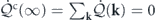 according to the total steady-state energy balance equation.
From the nonequilibrium thermodynamic perspective based on the heat-bath reinterpretation, the constant energy flux across scales in the inertial subrange in turbulence energy cascade is simply the heat flow through the fluid system in the wavenumber dimension, which is conducted by the nonlinear convective force, but driven by the temperature difference of the heat baths in the two ends of the scales. Without the temperature difference (e.g., in the case of equilibrium fluids obeying detailed balance), there is no energy cascade across scales although the nonlinear convective force is still present. The temperature difference of the heat baths in the large and small scales provides the working condition for the nonlinear convective force to do its job of conducting energy from the large scales to the small scales in the form of turbulence energy cascade.
5.3.5. The second law of thermodynamics in turbulence energy cascade
Turbulence energy cascade is a typical nonequilibrium irreversible process. From the thermodynamic perspective, the extent of detailed balance breaking and nonequilibrium irreversibility in the turbulence energy cascade process can be quantitatively measured by the steady-state entropy production rate  . Positive steady-state entropy production is a manifestation of the second law of thermodynamics at nonequilibrium steady states. Entropy production and entropy flow are balanced at the steady state. We use the expression of the entropy flow rate to calculate the entropy production rate:
  .
.
We will not do an accurate calculation as that requires the knowledge of the steady-state probability distribution functional Ps[u] which is difficult to obtain. Semi-quantitative results will be presented in the following, based on estimates in the three regions of the wavenumber dimension. In the energy injection range, the entropy production can be estimated as

where we have used equations (45) and (46). In the energy dissipation range, the entropy production can be estimated as

where we have used equation (47) and estimated the temperatures in the dissipation range with that at the characteristic wavenumber kη
. In the inertial subrange, the entropy production can be neglected as  . Typically,
  , especially for high Reynolds numbers. Hence, only
  need to be retained. We thus finally obtain the entropy production rate per unit mass:

Consider the infinite Reynolds number limit represented by ν → 0. In this limit, the Kolmogorov length scale η → 0, which means kη → ∞, leading to Teff(kη ) → 0, and as a consequence,

That is, the entropy production rate per unit mass diverges in the infinite Reynolds number limit.
The infinite Reynolds number limit corresponds to the case that the temperature difference between the large and small scales becomes infinitely large. The divergence of entropy production is a manifestation and reflection of this extreme nonequilibrium condition on the thermodynamic level. The steady-state entropy production quantifies the degree of detailed balance breaking, non-Gaussian statistics and time irreversibility, as shown by its expressions in equation (38) in relation to the nonequilibrium trinity. The divergence of entropy production implies that the extent of detailed balance breaking, non-Gaussian statistics and time irreversibility is extreme. It is intuitive that, in the case of an infinite temperature difference, the heat conduction in the wavenumber dimension, representing turbulence energy cascade, becomes completely time irreversible. The connection of time irreversibility and non-Gaussian statistics in the nonequilibrium trinity then implies that the statistics of the fluid system in this extreme nonequilibrium case is utterly different from the Gaussian statistics. Both aspects are consequences of detailed balance breaking generated by the infinite temperature difference, manifested on the thermodynamic level as divergent entropy production.
6. Conclusion
In this article, we have established the nonequilibrium thermodynamics for stochastic fluid systems and turbulence using the potential landscape and flux field theory, based on a reinterpretation of the stochastic fluid system as an interacting many-body system in contact with multiple heat baths in the wavevector space. A set of nonequilibrium thermodynamic equations has been constructed for general stochastic fluid systems, which remains valid for turbulence in the far-from-equilibrium regime. The Gaussian cross entropy balance equation is a new thermodynamic equation that relates the first law with the second law of thermodynamics and connects detailed balance breaking to entropy flow and entropy production at the steady state. We have demonstrated that temperature nonuniformity breaks detailed balance, leading to the nonequilibrium trinity that characterizes the nonequilibrium irreversible nature of the fluid system, which further results in steady-state entropy production and energy flow. From the thermodynamic viewpoint, turbulence energy cascade has the intuitive interpretation of heat conduction in the wavenumber dimension, with the energy flow across scales conducted by nonlinear convection and driven by the temperature difference between the large and small scales. The nonequilibrium irreversibility of turbulence energy cascade is quantified by the steady-state entropy production rate. The major findings in this work can be summarized by equations (26)–(36) and the figures.
In the future we plan to continue the mutually beneficial dialogue between fluid dynamics and nonequilibrium statistical physics. Transfer of ideas between these two fields may lead to a cascade of insights that are inaccessible in one field alone and prove to be fruitful for both fields. The nonequilibrium thermodynamics established in this work for fluid turbulence may be further developed into a more complete nonequilibrium statistical theory applicable to more general nonequilibrium systems in physics, chemistry and biology. In turn, we hope that the extended theoretical framework may one day help us better understand the real-world fluid turbulence. The present turbulence thermodynamics is still built on a highly simplified model, namely statistically homogeneous and isotropic turbulence generated by stochastic forcing. Some directions of extension may bring the theory closer to the real-world scenario. For instance, the conditions of statistical homogeneity and isotropy can be relaxed by assuming more general forms of stochastic forcing. Colored noise and non-Markovian dynamics may also be considered. Deterministic forcing can be obtained from the stochastic forcing setting by taking the small noise limit. More realistic boundary conditions can be used. Compressible fluids may also be incorporated into the framework. There is another issue worth further investigation. The nonequilibrium thermodynamics in this article is built for the hydrodynamic modes of the fluid, which is different from the standard fluid thermodynamics for the molecular degrees of freedom. A unifying framework that clarifies the connection between them is obviously desirable. These issues as well as others will be explored in the future.
Acknowledgments
WW is supported by the National Natural Science Foundation of China (Grant Nos. 11905222 and 21721003).
Appendix A.: Physical space representation of the nonequilibrium thermodynamics
The nonequilibrium thermodynamics in section 4 can be reformulated in the physical space.
We first note that, according to equations (8) and (9), Ds(k) = Πs(k)νk2 Teff(k)/L3. Transformed back to the physical space, this means Ds(x − x') = Πs(∇)[−νΔTeff(x − x')], where Teff(x − x') = ∑k Teff(k)eik⋅(x−x ')/L3. In general, the effective temperature becomes a two-point function Teff(x − x') in the physical space. This is because the stochastic force in general has nonlocal spatial correlations characterized by Ds(x − x') that is not delta-correlated. In the particular equilibrium case with Teff(k) = Teff, we have Teff(x − x') = Teff δ(x − x'), which means Teff is also the global temperature in the physical space.
The Fokker–Planck equation and the nonequilibrium trinity in section 3 can also be formulated in the physical space [52]. Following a line of derivation similar to that in section 4, with certain adaptations, the same set of nonequilibrium thermodynamic equations in equation (26) can be obtained in the physical space representation:

where the expressions of the thermodynamic quantities in the physical space representation are given below:


where ![${T}_{\text{eff}}^{-1}\left(\mathbf{x}-{\mathbf{x}}^{\prime }\right)={\sum }_{\mathbf{k}}{\text{e}}^{\text{i}\mathbf{k}\cdot \left(\mathbf{x}-{\mathbf{x}}^{\prime }\right)}/\left[{T}_{\text{eff}}\left(\mathbf{k}\right){L}^{3}\right]$](https://content.cld.iop.org/journals/1367-2630/22/11/113017/revision3/njpabc7d2ieqn147.gif) and
and ![${\mathbf{D}}_{\mathrm{s}}^{-1}\left(\mathbf{x}-{\mathbf{x}}^{\prime }\right)={\sum }_{\mathbf{k}}{\text{e}}^{\text{i}\mathbf{k}\cdot \left(\mathbf{x}-{\mathbf{x}}^{\prime }\right)}{\mathbf{\Pi }}^{\mathrm{s}}\left(\mathbf{k}\right)/\left[\nu {k}^{2}{T}_{\text{eff}}\left(\mathbf{k}\right){L}^{3}\right]$](https://content.cld.iop.org/journals/1367-2630/22/11/113017/revision3/njpabc7d2ieqn148.gif) . The equivalence of the expressions in equations (A2)–(A10) and those in equations (28)–(34) can be shown with Fourier analysis.
. The equivalence of the expressions in equations (A2)–(A10) and those in equations (28)–(34) can be shown with Fourier analysis.
Appendix B.: Necessary and sufficient condition for detailed balance
We prove the following theorem presented in the main text in section 4.6.
Theorem. The necessary and sufficient condition for detailed balance, namely B[u] = 0 for all velocity fields in the state space, is that the effective temperature distribution Teff(k) (k ≠ 0) is uniform.
Proof. The sufficient condition is obvious according to equation (37). We only need to prove the necessary condition. The strategy is to choose suitable velocity fields in a systematic way, so that the constraints on Teff(k) dictate that it has to be uniform. We choose a class of velocity fields with nonvanishing values at only three pairs of wavevectors, ±k1, ±k2, and ±(k1 + k2), where k1 and k2 are linearly independent. For these velocity fields, the expression of B[u] in equation (37) reduces to
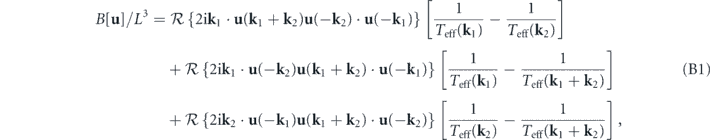
where we have used k ⋅ u(k) = 0. Then we choose a more specific velocity field with its values assigned as follows:

The prefactors νL and ν are added for dimensional reasons. This velocity field satisfies u*(k) = u(−k) and k ⋅ u(k) = 0 required to be in the state space. Direct calculations then yield:  ,
,  , and
, and  , where θ is the angle between k1 and k2. Therefore, according to equation (B1), B[u] = 0 for this particular velocity implies that Teff(k2) = Teff(k1 + k2). Similarly, by switching the roles of k1 and k2, it can be shown that Teff(k1) = Teff(k1 + k2). Thus when detailed balance holds,

for k1 and k2 that are linearly independent. Geometrically, this means for any three wavevectors forming a triangle, their effective temperatures are the same when detailed balance holds. Given the form of the wavevector k = (2π/L)(n1, n2, n3), it is then easy to show, using basic wavevectors and their combinations, that when detailed balance holds, Teff(k) at all wavevectors have to be the same except for k = 0. We have thus proven the necessary condition for detailed balance and the theorem.□