


Abstract
The effective lifetime of a quantum state can increase (the quantum Zeno effect) or decrease (the quantum anti-Zeno effect) in the response to increasing frequency of the repeated measurements and the multiple transitions between these two regimes are potentially possible within the same system. An interesting question arising in this regards is how to choose the optimal schedule of repeated measurements to achieve the maximal possible decay rate of a given quantum state. Addressing the issue of optimality in the quantum Zeno dynamics, we derive a range of rigorous results, which are, due to generality of the theoretical framework adopted here, applicable to the majority of models appeared in the quantum Zeno literature. In particular, we prove the universal dominance of the regular stroboscopic sampling in the sense that it always provides the shortest expected decay time among all possible measurement procedures. However, the implementation of the stroboscopic protocol requires the knowledge of the optimal sampling period which may depend on the fine details of the quantum problem. We demonstrate that this difficulty can be overcome with the tricky non-regular measurement schedule inspired by the scale-free restart strategy used to speed up the completion of the probabilistic algorithms and Internet tasks in computer science as it allows to achieve a near-optimal decay rate in the absence of detailed knowledge of the underlying quantum statistics. Besides, our general approach reveals unexpected universality displayed by the quantum systems subject to the optimally tuned rate of Poissonian measurements and the simple statistical criteria to discriminate between Zeno and anti-Zeno regimes following from this universality. We illustrate our findings with an example of Zeno dynamics in the system of optically-trapped ultra-cold atoms and discuss the implications arising from them.
Export citation and abstract BibTeX RIS

Original content from this work may be used under the terms of the Creative Commons Attribution 4.0 licence. Any further distribution of this work must maintain attribution to the author(s) and the title of the work, journal citation and DOI.
1. Introduction
As was recognized soon after establishing the foundations of the quantum theory, the repeated measurements can slow down the quantum evolution, e.g., inhibit the spontaneous decay of an unstable system. In the idealized limit of infinitely frequent instantaneous measurements the quantum transitions are completely suppressed so that the system is frozen to the initial state. This phenomenon had first been qualitatively described by computer science pioneer Alan Turing [1] and later took the name of the quantum Zeno effect [2]—after ancient Greek philosopher Zeno of Elea famous for his paradoxes challenging the logical possibility of motion.
During past decades the measurement-induced slow down of quantum evolution has been investigated for a variety of experimental setups [3–11]. Importantly, the opposite phenomenon—the quantum anti-Zeno effect or inverse Zeno effect [12, 13]—has also been demonstrated experimentally [14, 15]. Quite often the effective decay rate exhibits a non-monotonic behavior in dependence on the measurement frequency (see, e.g., references [16, 17]) so that both the quantum Zeno and anti-Zeno effects can potentially be observed in the same system. This open the door to the opportunity to optimize the rate of quantum transitions by the carefully scheduled repeated measurements. However, it remains unclear if there are any general guiding principles to design the optimal measurement schedule providing the fastest decay of a quantum state of interest.
Besides, considerable theoretical efforts have been made to find the conditions to discriminate between the quantum Zeno and the anti-Zeno effects in the decay of unstable systems. Say, accordingly to references [13, 16, 18] one should explore the general features of the system–environment interaction and calculate the residue of the propagator involving the environmental spectral density function. More recently, in reference [19] an explicit analytical criterion is derived which relates the sign of Zeno dynamics of the two-level system in a dissipative environment with the convexity of the spectrum. While these theoretical approaches provide a valuable insight, one may ask how to formulate the general criteria (if any) of the Zeno and anti-Zeno regimes in terms of the directly measurable decay statistics at a given measurement frequency, i.e. without referring to any details of the interaction Hamiltonian.
To address these challenges, here we develop a unifying theoretical approach to the quantum Zeno dynamics for a generic quantum system under an arbitrary distributed measurement events. Our analysis focuses on the behavior of the average time required to detect the decay of an initial state in the series of successive measurements. This metric exhibits a non-monotonic behavior in dependence on the measurement frequency so that one can achieve the optimal decay conditions by bringing the system to the point of Zeno/anti-Zeno transition. With simple arguments, we determine the optimal detection strategy which provides the shortest expected decay time: one should apply measurements in a strictly periodic manner, i.e. each τ* units of time. Since the optimal measurement period τ* of such a stroboscopic protocol depends on the parameters of the particular quantum system, which may be poorly specified, we next propose the non-uniform measurement protocols whose performance is weakly sensitive to such details. These protocols resemble the scale-free restart strategies previously developed to improve the mean completion time of the random search tasks [20, 21] and of the probabilistic algorithms in computer science [22]. Finally, our general framework is used to describe the peculiarities of the Zeno/anti-Zeno transition in the practically important case of randomly distributed Poissonian measurement events. It is shown that quantum decay under optimally tuned rate of Poissonian measurements exhibits universal statistical features allowing us to formulate the simple and widely applicable criteria to discriminate between Zeno and anti-Zeno regimes. All these findings are illustrated with the example of Zeno dynamics in the interband Landau–Zener tunneling of ultra-cold atoms [14, 23].
2. Theoretical framework
In the description of quantum Zeno dynamics a key role is played by the survival probability P(T), i.e. the probability of finding the quantum system in its initial state after time T has elapsed in the absence of any measurements performed on the system prior to this point in time. We are interested in the scenario, when the system undergoes a series of measurements during the time evolution to check whether it is still in the initial state. Explaining the general idea of our approach, we will treat the measurements as instantaneous projections which is justified when the time required to perform a measurement is small compared to the typical inter-measurement interval. However, as explained through the text, the main conclusions of our analysis survive in the more general settings with non-negligible measurement duration. Note also, we assume that the system–environment correlations can be neglected, which implies that the survival probability after several measurements factorizes.
The measurement protocol is characterised by the sequence of the inter-measurement time intervals  . In what follows, we calculate the expectation of the random time t when the measurement attempts finally result in detection of decay. This quantity can be determined from the infinite chain of equations


where  is the binary random variable which is equal to zero if the outcome of the kth measurement is 'yes' (i.e. the decay of the initial state is detected) and is unity otherwise, and ti represents the time remaining to the decay provided the ith measurement was 'no' (i.e. the decay is still not detected). Intuition behind this set of equations is very simple: if the next measurement attempt failed to detect decay, the system quantum evolution starts anew from the initial (undecayed) state. Performing averaging over the quantum statistics and taking into account that
  one obtains

The later equation relates the expectation of the decay detection time to the quantum survival probability of the system. Once P(t) is known, equation (4) allows to calculate the expected decay time for any sequence of the inter-measurement intervals  . Let us discuss how this formula simplifies for the particular measurement strategies most studied in the existing literature. In the original formulation of the quantum Zeno effect [2], the measurement protocol was stroboscopic, i.e. the measurement events are equally spaced in time,
  . In this case, the right-hand side of equation (4) represents the sum of the infinite geometric series with the common ratio P(τ) so that we readily find

Another important scenario is the stochastic measurements protocol where measurement events are separated by random time intervals [24–28]. In this case, Ti's are assumed to be independent and identically distributed random variables sampled from the probability density ρ(T) with the well-defined first moment  . To calculate the expected decay time, we should additionally average equation (4) over the statistics of inter-measurement intervals. This gives

Clearly, the stroboscopic protocol with period τ can be treated as a particular case of randomly distributed protocol having measurement intervals distribution ρ(T) = δ(T − τ).
Importantly, while here we consider the mean detection time as the key metric of interest, the previous theoretical studies of Zeno effect focused mainly on the calculation of the effective decay rate extracted from the behavior of the measurements-modified survival probability, see, e.g., [16, 17, 19, 29–31]. Say, for the stroboscopic measurement protocol with period τ, the probability of finding the system in its initial state after N measurements (i.e. after time t = Nτ) is equal to P(τ)N = e−Γt, where Γ = −ln P(τ)/τ is the effective decay rate. In more general situation with stochastic measurement protocol, the survival probability after N measurements is given by  . Due to the law of large numbers, for N ≫ 1 this probability is equal to e−Γt, where t = N⟨T⟩ and
  . Obviously, when the measurement frequency is high enough, deviation of P(T) from unity for typical values of T is small and we can safely replace ⟨ln P(T)⟩ ≈ 1 − ⟨P(T)⟩. Then, using equation (6), one obtains Γ ≈ (1 − ⟨P(T)⟩)/⟨T⟩ = ⟨t⟩−1, i.e. the mean decay time is equal to the inverse effective decay rate. Thus, these two approaches to quantification of Zeno dynamics—either in terms of the effective decay rate, or in terms of the expected decay time—become equivalent in the limit of sufficiently frequent measurements. Note also that the mean detection time is more natural and well-defined metric while dealing with the non-uniform measurement protocols discussed below.
The behavior of ⟨t⟩ as a function of ⟨T⟩ allows us to identify the Zeno and anti-Zeno regimes. Namely, the expected decay time can either increase with decreasing ⟨T⟩, which we refer to as the Zeno effect, or decrease for more frequent measurements, which we define as the anti-Zeno effect. Equivalent definition of Zeno and anti-Zeno effects in terms of effective decay rate was adopted, e.g., in references [12, 17, 29, 32, 33]. In general, ⟨t⟩ in its dependence on ⟨T⟩ must exhibit a minimum corresponding to the Zeno/anti-Zeno transition. This is particularly evident in the case of the stroboscopic measurements. At the very beginning of the decay 1 − P(τ) ∝ τ2 [34] and therefore ⟨tτ⟩ ∝ 1/τ, whereas for the very large detection period ⟨tτ⟩ ∝ τ (assuming that P(τ) → 0 as τ → ∞). Thus, the dependence of mean time required to detect the decay on the stroboscopic period always attains a minimum, see the right panel in figure 1. Note also that multiple Zeno/anti-Zeno transitions (i.e. multiple local extrema of ⟨t⟩ or Γ) may occur, see, e.g., references [17, 29].

Figure 1. The cartoon schematic of the decay time measurement in quantum tunneling experiment (left). The expected time required to detect the decay in a series of stroboscopic measurements attains a minimum corresponding to the Zeno/anti-Zeno transition (right).
Download figure:
Standard image High-resolution image3. Optimality of the stroboscopic protocol
For the sake of illustration, we will consider a system consisting of ultra-cold atoms that are trapped in an accelerating periodic optical potential of the form V0 cos(2kLx − kLat2), where V0 is the potential amplitude, kL is the laser wavenumber, x is position in the laboratory frame, a is the acceleration and t is time—the experimental setup intensively discussed in references [14, 23]. In the accelerating reference frame, x' = x − at2/2, this potential becomes V0 cos(2kLx') + Max', where M is the mass of atoms and the last term corresponds to the inertial force experienced by them. The energy spectrum of the considered system under the assumption of zero acceleration consists of Bloch bands separated by gaps. As an initial condition, we assume that the lowest band is uniformly occupied, while the higher bands are empty. When an acceleration is imposed, the atomic quasimomentum changes as the atoms undergo Bloch oscillations. The trapped atoms can escape from the accelerating lattice by interband Landau–Zener tunneling. The corresponding escape probability can be calculated analytically (see equation (A1) in appendix

Figure 2. The probability P(t) of finding the trapped atom in its initial state as a function of time t for different potential amplitudes V0. The acceleration of optical potential is equal to a = 0.1. Here and in what follows we measure the time t in units of  , the potential amplitude V0 in
  , and acceleration a in
  .
.
Download figure:
Standard image High-resolution imageIn figure 3(a) we plot the expected tunneling time ⟨t⟩ as a function of mean inter-measurement intervals ⟨T⟩ for various stochastic measurement strategies having uniform in time statistics. We see that a minimum of ⟨t⟩ is always achieved and while the values taken by the different minima and their positions depend on the distribution of the inter-measurement time, it is the regular stroboscopic protocol that provides the lowest of minima. Also, figure 3(b) demonstrates that the stroboscopic protocol outperforms the non-uniform in time measurement procedures.

Figure 3. (a) The mean time to decay ⟨t⟩ as a function of mean detection period ⟨T⟩ for various uniform in time stochastic measurement strategies demonstrates dominance of the regular stroboscopic sampling. (b) The stroboscopic protocol also outperforms the geometric and the stochastic scale-free measurement protocols which are non-uniform in time (see section 4.1 for the definition of these measurement strategies). The survival probability P(T) defined by equation (A1) is taken for a = 0.1 and V0 = 0.4, the initial time-step for geometric protocol is τ0 = 0.01.
Download figure:
Standard image High-resolution imageThese observations allow us to conjecture that in the case of ultra-cold atoms, the stroboscopic protocol is the optimal measurement strategy. Importantly, this is also true in general. For the rigorous proof, assume that τ* is the optimal period of the stroboscopic measurement protocol minimizing the mean time to decay which is given by equation (5), i.e.

for all 0 < τ < ∞. Below we show that for any other measurement procedure  the resulting expected decay time ⟨t⟩ cannot be lower than
  . Indeed, from equation (4) one obtains

Next, we note that 1 − P(T1) is the probability to register the decay after the first measurement Q1, and accordingly,  is the probability of registering the decay after the nth measurement. Also, we remind that
  is the expected decay time under stroboscopic protocol of period Tn, and, therefore,

Further we exploit the facts that  (direct consequence of equation (B3) and normalization condition
  ) to obtain from equation (9)

This proves that stroboscopic measurement protocol is optimal among all possible strategies.
The same conclusion can be drawn from the following qualitative arguments. Let  be the optimal measurement schedule for a given quantum system and assume that the outcome of the first measurement is 'no'. Clearly, by the definition of the optimal strategy, the subsequent measurements must minimize the residual time to decay. Since the system's quantum evolution starts anew after the first measurement, the sequence of the inter-measurement intervals
  minimizing the remaining time to decay coincides with the original sequence
  . This means that the optimal sampling protocol is strictly periodic, i.e.
  . Note that these simple arguments do not invoke any system-dependent features and remain valid in the case of non-instantaneous measurements, thus making our conclusion completely universal.
In figure 4 we compare the behavior of the mean decay time ⟨t⟩ and of the inverse decay rate Γ−1 in their dependence on the measurement period T for the stroboscopic measurement protocol. While both metrics attain minimum at very close optimal values of T, the match of two curves is not perfect (especially for large measurement periods), and, so, it is natural to ask if there is a rigorous proof that the stroboscopic strategy is optimal when one wish to maximize the effective decay rate Γ. We provide such a proof in appendix
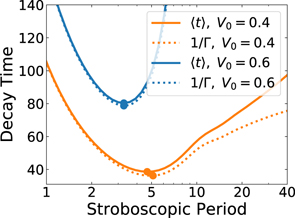
Figure 4. The mean time to decay ⟨t⟩ = T/(1 − P(T)) and the inverse decay rate 1/Γ = −T/ln P(T) as a function of detection period T for stroboscopic measurements demonstrate that the transition point between Zeno and anti-Zeno regimes weakly depends on the choice of the quantifying metric. The difference between the curves decreases as P(T) approaches unity, i.e. at sufficiently small values of T. The survival probability P(T) defined by equation (A1) is taken for V0 = 0.4 (orange curves) or V0 = 0.6 (blue curves) and a = 0.1.
Download figure:
Standard image High-resolution image4. Benefits of the scale-free measurement protocols
4.1. Luby-like protocol
As we learn from consideration in the previous section, to achieve the maximal decay rate one should implement the stroboscopic measurements with carefully tuned sampling period τ* which, strictly speaking, may depend on the fine details of the underlying quantum process. An interesting question then naturally emerges: is it possible to have a realization of the measurement sequence that gives value of the expected decay time close to the optimal value ⟨ ⟩ without detailed knowledge of the system parameters? Previously, a similar challenge motivated the development of the universal restart strategy capable to improve the average running time of the Las Vegas type computer algorithms without introducing any assumptions regarding the completion time statistics [22]. Motivated by the appealing analogy between restart and projective measurement (indeed, the projection postulate tells us that at every moment one confirms the survival of the system through the measurement, the quantum state of the system is reset to the initial undecayed one and its evolution starts from scratch), we now investigate the effect of the Luby-like measurement protocol [22] on the quantum Zeno dynamics. Namely, we assume that the inter-measurement intervals are given by
  . The ith term in this sequence is

where the initial time step τ0 should be smaller then the (estimated) decay time of the quantum state under study.
This strategy possesses the following remarkable property: the total time spent on inter-measurement intervals of each possible length up to the end of some interval in the measurement schedule is roughly equal. Indeed, as follows from equation (11), all inter-measurement intervals are powers of two and each time a pair of intervals of a given length has been completed, an interval of twice that length is immediately executed. If the total time elapsed since the start of measurements is t ≫ τ0, then approximately  different measurement periods have been applied, and the total time spent on each is
  . This means that the effective probability density, describing the relative frequencies of appearance of the different measurement periods in the sequence defined by equation (11), behaves in the scale-free fashion:
  , where Tk = 2k−1τ0. Due to this property, the strategy does not introduce any characteristic time scale into the measurement process.
It turns out that the Luby-like measurement strategy allows to come surprisingly close to the optimum value of the mean decay time provided by the best stroboscopic protocol. Namely, in appendix

which is universally valid for any quantum state whose survival probability P(t) is a monotonically decreasing function. Here  and
and  . Thus, the decay of a quantum system under the Luby-like strategy is only a logarithmic factor slower than the decay of the same system subject to the optimally tuned stroboscopic measurements.
Importantly, in practice the performance of this measurement procedure is much better that the upper bound predicted by equation (12), see figure 5. This is because in derivation of equation (12) we were struggling mainly for the logarithmic factor and did not try to reduce the numerical constants C1 and C2 in the involved estimates. Note also that the account of the non-zero measurement duration changes the constant C1, while the structure of the final answer remains the same (see appendix

Figure 5. The comparison of the Luby-like measurement strategy with the optimal stroboscopic protocol for different values of the potential amplitude. The acceleration of optical potential is equal to a = 0.1. The black dashed line is defined only for the sufficiently small values of potential amplitude, since larger V0 lead to non-monotonic behavior of the survival probability P(T), thus, violating the assumptions underlying the proof of equation (12).
Download figure:
Standard image High-resolution image4.2. Other scale-free protocols
Next we introduce a class of non-uniform measurement protocols resembling the scale-free restart strategies recently proposed for the robust optimization of the mean first-passage time in random search processes [20, 21]. These strategies are effective for the problems where the survival probability has the form P(T) = f(T/T0), where T0 is the unknown characteristic time associated with quantum evolution.
Assume that the measurements are applied at random time moments at rate which is inversely proportional to the time elapsed since the start of the experiment, i.e. r(t) = α/t, where α is a dimensionless constant [20]. As we see in figure 6(a), such measurement protocol does not need to be optimized with respect to the characteristic time scale T0 of the underlying quantum problem: the mean decay time as a function of α attains its minimum at optimal value α* which is determined by the particular form of the function f(T/T0), but does not depend on the time scale T0. The mathematical explanation of this observation can be found in appendix

Figure 6. Demonstration that the optimal values of strategy parameters do not depend on the characteristic time scale T0 for scale-free (a) and geometric (b) protocols, τ0 = 0.01. The involved survival probabilities are ![${P}_{A}=\mathrm{exp}\left[-{\left(T/{T}_{0}\right)}^{2}\right]$](https://content.cld.iop.org/journals/1367-2630/22/7/073065/revision2/njpab9d9eieqn29.gif) ,
, ![${P}_{B}=1/\left[1+{\left(T/{T}_{0}\right)}^{2}\right]$](https://content.cld.iop.org/journals/1367-2630/22/7/073065/revision2/njpab9d9eieqn30.gif) , and
, and ![${P}_{C}=\left[1+\frac{T/{T}_{0}}{1+{\left(T/{T}_{0}\right)}^{2}}\right]\mathrm{exp}\left[-T/{T}_{0}\right]$](https://content.cld.iop.org/journals/1367-2630/22/7/073065/revision2/njpab9d9eieqn31.gif) .
.
Download figure:
Standard image High-resolution imageThe same property is exhibited by the geometric protocol [21], see figure 6(b). Here the measurement time instants are chosen from the geometric sequence  , where τ0 ≪ T0 is the initial time-step and q is the dimensionless common ratio. Again the optimal value q* minimizing the expected decay time does not depend on the scale T0.
Thus, once the form of the survival probability f(T/T0) is known, one can optimize the quantum evolution using the scale-free sampling of the measurement times even in the absence of reliable estimate of the characteristic time scale T0. An important open question, which is beyond of the scope of the current article, is how to derive the rigorous bounds on the performance of these measurement protocols.
5. Poissonian measurements
Sometimes the form of the measurement protocol is dictated by the very experimental conditions. Say, in some settings, the measurement process is of stochastic nature so that the time interval between two consecutive measurements is randomly varied [24, 26, 27]. A particularly important example is the Poissonian measurements for which the inter-measurement intervals are independently sampled from the exponential distribution, i.e. ρ(T) = re−rT, where r is the measurement rate. In this section we describe the universal statistical properties of quantum decay in the systems subject to the optimal measurement rate bringing the expected decay time to its extremum and discuss the practical implications arising from this universality.
In this case  and
and  , where
  denotes the Laplace transform of P(t) evaluated at r, so that equation (6) reduces to

To arrive at the model-independent manifestations of the Zeno/anti-Zeno transition announced above, one also needs to calculate the second statistical moment of the random time required to detect a decay in a series of Poissonian measurements. Note that for any stochastic measurement schedule with uniform in time statistics, the random times t and t1 entering equation (1) are the statistically independent copies of each other. In other words, the time to decay satisfies the simple renewal equation: t = T + t'xT, in which xT is the binary random variable which is equal to zero if the outcome of the first measurement is 'yes' and is unity otherwise, T is the random measurement time sampled from ρ(T), and t' is independent copy of t. Therefore, t2 = T2 + 2t'xTT + t'2xT, and after averaging over the statistics of T and over the quantum statistics one obtains ⟨t2⟩ = ⟨T2⟩ + 2⟨t'xTT⟩ + ⟨t'2xT⟩. Since ⟨t'xTT⟩ = ⟨t'⟩⟨xTT⟩, ⟨t'2xT⟩ = ⟨t'2⟩⟨xT⟩, ⟨t⟩ = ⟨t'⟩ and ⟨t2⟩ = ⟨t'2⟩, we then readily find

For the measurement events coming from Poisson statistics,  ,
,  ,
,  , and ⟨t⟩ is given by equation (13). Substituting these expressions into equation (14) gives the following result for the second moment of the decay time

Now let us assume that we found the optimal measurement rate r* such that the expected decay time of the initial quantum state attains its (local or global) extremum. Then  , and equation (13) together with equation (15) yield

No assumptions were made concerning the particular form of the survival probability P(T) and, thus, equation (16) must hold for an arbitrary quantum system subject to optimally tuned Poissonian measurements. Interestingly, equation (16) is automatically valid for any quantum decay process subject to the strictly periodic repeated measurements with the period  . Indeed, for ρ(T) = δ(T − τ), equation (14) reduces to
  , where ⟨tτ⟩ is given by equation (5), and, therefore,
  . Thus, the quantum decay altered by the optimal Poissonian measurements approaches in its statistical properties the quantum decay under the stroboscopic measurements characterised by the twice larger (in average) sampling period.
The point of the Zeno/anti-Zeno transition associated with the optimal rate of Poissonian measurements is also characterized by another universal statistical relation

in which the time  has the following meaning. Assume that we apply a single projective measurement at the random (Poisson) moment of time to each of the large number of identically prepared quantum systems. Then
  is the average time of those trials that gave the outcome 'yes'. To derive equation (17) let us note that, as follows from equation (13),
  where
where  is the Laplace transform of the function Q(T) = 1 − P(T) evaluated at r. Obviously, Q(T) represents the probability that the initial quantum state will decay after time T. For r = r* one has
  so that
  . Introducing the time
  we arrive at equation (17).
The universal identities described above allow us to formulate the simple and practically important criteria to distinguish between the quantum Zeno and the anti-Zeno effects in terms of the directly measurable statistics of the random decay time. Namely, one can determine the sign of the Zeno dynamics by probing the deviations from equations (16) and (17): it is straightforward to show from equations (13) and (15) that the conditions  (or
(or  ) and
) and  (or
(or  ) indicate the Zeno (∂r⟨tr⟩ > 0) and anti-Zeno (∂r⟨tr⟩ < 0) regimes, respectively, see figure 7 for the illustration. Let us stress that equations (16) and (17) were derived assuming that the inter-measurement intervals are taken from the exponential distribution and, for this reason, these criteria are universally valid only in the case of Poissonian measurements.

Figure 7. Statistical properties of the decay detection time for the Landau–Zener tunneling of ultra-cold atoms trapped in an accelerating periodic optical potential (a = 0.1 and V0 = 0.4) and subject to Poissonian measurements. The optimal measurement rate bringing the expected decay time ⟨tr⟩ to a minimum entails equations (16) and (17).
Download figure:
Standard image High-resolution image
Importantly, an assumption of instantaneous measurements does not play a crucial role for our argumentation. Relaxing this assumption and introducing a non-zero duration of the measurement event Δ we arrive at slightly modified identities characterising the Zeno/anti-Zeno transition (see appendix

and

which trivially reduce to equations (16) and (17) at Δ = 0. The criteria of the quantum Zeno effect in the presence of non-instantaneous Poissonian measurements are given by the inequalities  and
and  , whereas the similar relations with opposite inequality signs indicate the anti-Zeno regime.
6. Conclusion and outlook
The quantum Zeno effect is an intriguing topic attracting ongoing interest from both experimental [3–11, 14, 15, 35] and theoretical [12, 13, 16, 17, 19, 29–31, 36–43] sides. In contrast to majority of previous studies aimed to explore the peculiarities of Zeno dynamics in particular classes of systems, here we adopted the very general theoretical approach which allowed us to address the broad optimization questions and the issue of universality.
Our analysis proves that the regular stroboscopic sampling—the most popular measurement protocol in the quantum Zeno research literature—is a universally optimal strategy providing the best performance (i.e. the shortest expected decay time in the point of Zeno/anti-Zeno transition) for any given quantum system, see section 3. However, in general, finding of the optimal sampling rate is not a simple task. Here we proposed the computer science-inspired solution to this problem. As was first noticed more than two decades ago, restarting a task whose run-time is a random variable (e.g., a probabilistic algorithm or downloading a web page) may speed up its completion, but the optimal restart frequency depends on the running time distribution which is usually unavailable in practice [22, 44–47]. To circumvent this obstacle, the scale-free sampling of the inter-restart intervals has been suggested [20–22]. By noting a formal analogy between the projective measurement of a quantum system and the restart of a classical stochastic process [20, 21, 48–67], we demonstrated that the scale-free detection protocols help to achieve the near-to-optimal decay rate without prior knowledge of the system parameters, see section 4. These theoretical results are expected to be an important step toward a robust measurement-based control of quantum dynamics especially taking into account the fact that they are not sensitive to the assumption of instantaneous measurements as discussed in the text.
Also, the present analysis establishes the general statistical criteria to discriminate between Zeno and anti-Zeno regimes and to probe the optimal decay conditions in practice. As explained in section 5, this insight became possible due to the surprising universality of the Zeno/anti-Zeno transitions under the Poissonian measurements: the extrema in the expected decay time as a function of the measurement rate entail the universal footprints in the decay statistics, see equations (16) and (17). Another remarkable consequence of this universality is the previously unknown inequality constraint relating the optimal (mean) sampling period  and the resulting expectation of the decay time
  . Indeed, since
  , we immediately find from equation (16) that
  . This also means that the average number of measurement attempts required to detect the decay, ⟨nr⟩ = r⟨tr⟩, is bounded from below in the point of the Zeno/anti-Zeno transition:
  . The broad model-independent nature of these conclusions should facilitate their experimental testing.
Besides the issue of optimal control of the quantum decay, another promising application of the above theory lies in the fields of quantum walks and quantum search algorithms. Assume that the quantum particle undergoes a unitary evolution and the series of measurements are performed (either in regular or in random fashion) to see if the particle has reached the target region of its phase space. What is then the expected time required to detect the first arrival of the particle? This question is known as quantum first detection problem [68–81], which is of basic notion for design of quantum search algorithms. As first noticed in reference [69], in some cases the optimum sampling period exists that brings the mean first detection time to the minimum thus providing opportunity to optimize the search process. We anticipate that the theoretical approach presented here may help to uncover the universal aspects of this kind of optimal behavior.
Acknowledgments
SB gratefully acknowledges support from the James S McDonnell Foundation via its postdoctoral fellowship in studying complex systems. VP acknowledges support from the Ministry of Science and Higher Education of the Russian Federation, program No. 0033-2019-0003. Authors would like to thank Yu. Makhlin for reading the manuscript and for providing useful comments.
Appendix A.: Escape probability of trapped atoms
To obtain a simple expression for the tunneling probability, one can keep only the gap between the first two Bloch bands, and neglect all the other bandgaps. This leads to a modified band structure with a single band, separated by a bandgap from free particle motion. This approximation is valid when the tunneling rate across the higher gaps is sufficiently high. By treating the non-adiabatic coupling between the trapped and non-trapped states as a weak perturbation, one can find that to leading order the logarithm of the survival probability in the trapped state is equal to [23]

where

and here we use dimensionless units introduced in the main text. In the parameter space of a and V0, the theory is valid inside the region bounded by the two curves  and
and  , and to the left of the line V0 = 1, see reference [82]. The presented expression demonstrates good agreement with experimental results and captures a short-term deviation from the exponential decay, see figure 2.
Appendix B.: Effective decay rate
Assume that τ* is the optimal period of stroboscopic measurement protocol maximizing the effective decay rate Γ(τ) = −ln P(τ)/τ, i.e.

for all 0 < τ < ∞. Let us multiply both sides of equation (B3) by  , where T > 0 is a random variable having probability density ρ(T),

Next we replace τ by T and average over statistics of T

On the left we see the decay rate  attained by the optimal stroboscopic measurement protocol, while the right-hand side represents the decay rate Γ for a system subject to measurements at a generally distributed random time moments (see introduction). This proves that stroboscopic measurement protocol is an optimal strategy in terms of maximization of the effective decay rate.
Appendix C.: Luby-like protocol
In our derivation of equation (12) we follow the line of argumentation originally proposed in reference [22] in the context of probabilistic algorithms under restart. We also show how these arguments can be generalized to account the non-instantaneous measurements.
For any j, if the total time spent on the inter-measurement intervals of duration 2jτ0 up to the end of some interval in the measurement schedule defined by equation (11) is W, then at most log2W/τ0 + 1 different intervals have so far been used, and the total time spent on each one cannot exceed 2W. Thus the total time elapsed since the start of the experiment up to this point is at most 2W(log2W/τ0 + 1).
As in the main text, we denote as τ* ≫ τ0 the optimal period of the stroboscopic measurement protocol minimizing the mean decay time given by equation (5). We set i0 = ⌈ log2(τ*/τ0)⌉ and m0 = ⌈ log2(1/Q(τ*))⌉, where Q(T) = 1 − P(T) and ⌈...⌉ denotes the procedure of rounding up to an integer. Consider the instant when  inter-measurement intervals of duration
  have elapsed. The probability that the corresponding measurements have not detected the decay of the initial state is at most

where we have used an assumption that the survival probability P(T) is monotonically decreasing function. At this point, the total time spent on intervals of duration  is
is

due to equations (5) and (B3), and by the observation above the total time spent up to this point is at most 2W(log2W/τ0 + 1). More generally, after  intervals of length
  have elapsed, the probability that the system has failed to decay is at most e−k, and the total time spent up to this point is at most 2kW(log2(kW/τ0) + 1). Therefore, the expected decay time of a quantum system subject to the Luby-like measurement protocol obeys the inequality

Taking into account equation (C2) and relation  one readily obtains equation (12).
Now let us introduce a non-zero duration of the measurement event, Δ. As previously, if the total time spent on the inter-measurement intervals of length 2jτ0 up to the end of some interval in the Luby sequence is W, then at most log2W/τ0 + 1 different intervals have so far been used, and the total time spent on each one cannot exceed 2W. The total time elapsed since the start of the experiment up to this point is at most  , where we accounted that each measurement entails a time penalty Δ. Denoting again as τ* ≫ τ0 the optimal period of the instantaneous stroboscopic measurements minimizing the mean decay time given by equation (5) and repeating the above argumentation we obtain

where  and
and  . Equation (C4) compares the performance of the non-instantaneous Luby measurements with that of the instantaneous stroboscopic measurements of the optimal period.
To proceed we note that the random time to decay t of a quantum system under the stroboscopic protocol with the inter-measurement period τ and the measurement duration Δ obeys the simple renewal equation: t = τ + Δ + xt', where x is the binary random variable decoding the outcome of the first measurement, and t' is independent copy of t. After averaging over the quantum statistics, one obtains the relation

which generalizes equation (5) to the case of non-instantaneous measurements. Let us denote as  the minimal expected decay time attained via optimization of equation (C5) over τ at a fixed value of Δ. As follows from equations (B3) and (C5),
  , where
  represents the optimal expected decay time in the limit of instantaneous measurements. The later inequality together with equation (C4) finally give us the bound

which tells us that, in the presence of an arbitrary time cost associated with non-zero measurement duration, the decay of a quantum system under Luby measurement strategy is a logarithmic factor slower than the decay of the same system subject to the optimally tuned stroboscopic measurements. Equation (C6) generalises equation (12) and reduces to it at Δ = 0.
Appendix D.: Stochastic scale-free protocol
Let us assume that the survival probability has the form P(T) = f(T/gT0), where T0 is the characteristic time associated with quantum evolution, and the dimensionless constant g represents the scale factor. We implement to this process the randomly distributed measurements at a non-uniform rate which is inversely proportional to the time elapsed since the start of the experiment, i.e. r(t) = α/t, where α is a dimensionless constant. This protocol is characterized by random scale-free time intervals between successive measurements. Namely, given a measurement at time t, the time till next measurement has the following distribution (see reference [20])

which implies that τ(t) has the same distribution as gτ(t/g). The remaining time to decay satisfies the following renewal equation

Using the observation above, we can rewrite this equation in the form

Thus, we see that

where the symbol ∼ means that the random variables have the same distribution. Taking the limit t → 0, we conclude that the decay time of the system subject to the scale-free measurements scales linearly with the characteristic time scale of the underlying quantum evolution. Therefore, the mean value is proportional to g, whereas the optimal parameter α*, which brings the expected decay time to a minimum, is insensitive to g.
Appendix E.: Non-instantaneous Poissonian measurements
Here we provide the technical details required to derive equations (18) and (19). Assume that the inter-measurement intervals are sampled from the exponential distribution, ρ(T) = re−rT, and each measurement takes time Δ. Then the random time to decay satisfies the following renewal equation: t = T + Δ + xTt', in which xT is the binary random variable which is equal to zero if the outcome of the first measurement is 'yes' and is unity otherwise, and t' is an independent copy of t. After averaging over the statistics of inter-measurement intervals and over the quantum statistics one obtains

Next, the same renewal equation yields t2 = T2 + Δ2 + 2TΔ + xTt'2 + 2TxTt' + 2xTt'Δ and after the procedure of averaging we find


It follows from equation (E1) that

and, therefore,

Substituting these expressions into equation (E3), after some algebra we obtain

For r = r* such as  , this relation gives us equation (18). Also it produces the criteria of the Zeno (∂r⟨tr⟩ > 0) and anti-Zeno (∂r⟨tr⟩ < 0) regimes discussed in the main text.
As for equation (19), let us introduce the time

which represents, by definition, the conditional mean decay time obtained if one averages the random decay detection time just over those realizations of the measurement process where the decay has been registered already in the first (Poissonian) measurement. Here, as before,  is the Laplace transform of Q(T) = 1 − P(T). From equation (E1) we find the expression

which yields equation (19) in the optimal point r = r* and gives us the conditions to discriminate between the quantum Zeno and the anti-Zeno effects.
Appendix F.: Numerical simulations
We use different numerical methods for the deterministic and stochastic measurement strategies. The simulations in the deterministic case were based on equation (4) and we interrupted the numerical summation over n when the survival probability  became less than
  = 10−10. We checked that a further increase in accuracy practically does not change the final results. In the stochastic case we simulated the behavior of ensemble of trapped atoms and collected statistics from at least N = 106 independent atoms.