


Abstract
We study the hydrodynamics and shape changes of chemically active droplets. In non-spherical droplets, surface tension generates hydrodynamic flows that drive liquid droplets into a spherical shape. Here we show that spherical droplets that are maintained away from thermodynamic equilibrium by chemical reactions may not remain spherical but can undergo a shape instability which can lead to spontaneous droplet division. In this case chemical activity acts against surface tension and tension-induced hydrodynamic flows. By combining low Reynolds-number hydrodynamics with phase separation dynamics and chemical reaction kinetics we determine stability diagrams of spherical droplets as a function of dimensionless viscosity and reaction parameters. We determine concentration and flow fields inside and outside the droplets during shape changes and division. Our work shows that hydrodynamic flows tends to stabilize spherical shapes but that droplet division occurs for sufficiently strong chemical driving, sufficiently large droplet viscosity or sufficiently small surface tension. Active droplets could provide simple models for prebiotic protocells that are able to proliferate. Our work captures the key hydrodynamics of droplet division that could be observable in chemically active colloidal droplets.
Export citation and abstract BibTeX RIS

Original content from this work may be used under the terms of the Creative Commons Attribution 3.0 licence. Any further distribution of this work must maintain attribution to the author(s) and the title of the work, journal citation and DOI.
Living cells are compartmentalized in order to organize their biochemistry in space. Many cellular compartments do not possess membranes and are formed by the assembly of proteins and RNA in compact condensates [1–16]. Such condensates often have liquid like properties and resemble droplets that form by phase separation of a complex mixture [1, 11–13]. Indeed protein droplets are observed to form in vitro by phase separation in physiological buffer [13, 15, 17–19]. Such droplets can organize chemical reactions in space, and the droplet dynamics can in turn be influenced by the reactions, as has been shown both in theory [8, 20–26] and experiments [13, 15, 17–19, 27, 28]. The ubiquitous nature of RNA-protein condensates in a large variety of different cells and organisms suggests that the physical chemistry of macromolecular phase separation represents an evolutionary old mechanism for the compartmentalization of chemistry and that droplet formation could have played a key role at the origins of life and the emergence of prebiotic protocells [15, 18, 29–40].
A minimal model of a protocell consists of a droplet that turns over by a chemical reaction and is constantly supplied with droplet material by diffusion from the outside [39]. In such a scenario droplets are maintained away from thermodynamic equilibrium and can reach a non-equilibrium steady state with a radius that is set by reaction parameters [26]. An interesting possibility is that the spherical shape of active droplets becomes unstable and droplets spontaneously divide in two smaller daughters drops, providing a physical mechanism for the division of prebiotic cells [39]. Such droplet dynamics is a hydrodynamic problem because surface tension in non-spherical droplets drives hydrodynamic flows that redistribute material and deform the droplet shape [41–44].
Here we develop a hydrodynamic theory of the dynamics of chemically active droplets. We show that chemical reactions in active droplets can perform work against surface tension and flows, giving rise to a shape instability that can result in droplet division. We investigate the conditions for which droplets divide and determine hydrodynamic flow fields of dividing droplets.
We consider an incompressible liquid consisting of droplet material B and solvent component A which can phase separate. The local composition is characterized by the concentration field c(x) of component B. Volume preserving chemical reactions can transform component A into component B and back,  . For simplicity, we first discuss an effective droplet model. A single droplet characterized by high concentration c of component B coexists with the surrounding fluid that mainly consists of A and contains B at low concentration, see figure 1. Both phases are separated by a sharp interface. The concentration of B satisfies a balance equation, where the chemical reaction provide a source or sink term s±(c),


Here, the indices + and − refer to quantities outside and inside the droplet, respectively. The flux  consists of advection by the fluid velocity
  and a diffusion flux, where D± denotes the diffusion constant of the droplet material in the two phases.

Figure 1. Chemically active droplet described by an effective droplet model. Shown is the concentration field c (blue and green color) of a stationary droplet (interface in black). Chemical reactions B → A create a sink of droplet material B in the droplet, and reactions A → B create a supersaturation  of droplet material in the A-rich phase outside. This creates concentration gradients of B, which drive diffusion fluxes of droplet material, while A flows in the opposite direction. The stationary droplet size results from the balance of the fluxes across the interface. (Parameters: = 0.176, A = 10−2, η+/η− = 1, k+/k− = 1, ν−/(k−Δc) = 1, D+/D− = 1, β− = β+,
  ).
).
Download figure:
Standard image High-resolution imageThe chemical reaction is described by the concentration-dependent rate  which in general is a nonlinear function of c. For simplicity, we linearize the chemical reaction rates in the vicinity of reference concentrations
  in each phase:

where  are the equilibrium concentrations that coexist at equilibrium across a flat interface. We have defined the reaction rate
  and the reaction constants
  . We focus on the case of positive coefficients
  and
and  , where B is produced outside the droplet, and degraded inside, see figure 1.
The hydrodynamic flow velocity  obeys Stokes equation of an incompressible fluid,

which accounts for momentum conservation ∂ασαβ = 0, where the stress tensor is given by σαβ = η± (∂αvβ + ∂βvα) − pδαβ. Here η± denotes the fluid shear viscosities inside and outside of the droplet. The pressure p plays the role of a Lagrange multiplier to impose the constraint  .
.
The bulk equations (1)–(4) are connected by boundary conditions at the droplet interface which we parameterize in spherical coordinates by the radial interface position R(θ, ϕ) as a function of the polar and azimuthal angles θ and ϕ. The stress boundary conditions read


where H(R) is the local mean curvature of the interface and γ is the droplet surface tension. The stresses at the interface on the inner and outer side of the droplet are denoted by  . The tensor indices n and t refer to tensor components normal and tangential to the interface, respectively. The normal and tangential tensor components are defined as
  and
and  , where nα is a unit vector normal to the surface and tα is a unit vector tangent to the surface. Equation (6) is valid for all tangent vectors and summation over repeated indices is implied. Using no-slip boundary conditions, the velocity field is continuous at the interface,

The concentration field c is discontinuous across the interface with values given by


which are set by the physics of phase coexistence and a local equilibrium assumption. The coefficients β± describe the effects of the Laplace pressure on the equilibrium concentrations at phase coexistence. In the presence of fluxes at the interface, the interface moves in normal direction. The radial growth velocity is

where  is a unit vector normal to the surface and
  is a unit vector in radial direction. Equation (10) captures both convection of the interface by flows and droplet growth and shrinkage by addition or removal of material.
We find non-equilibrium steady state solutions to equations (1)–(10) with a spherical droplet of stationary radius  and stationary concentration field
  , where r is the radial coordinate, see appendix A. The stationary pressure
  exhibits a jump
  across the interface and no hydrodynamic flows exist,
  . An example for a stable non-equilibrium steady state with steady state concentration profile inside and outside the droplet of radius
  is shown in figure 1.
We first discuss the properties of these stationary states as a function of external supersaturation  and the dimensionless reaction rate A = ν−τ/Δc inside the droplet. The supersaturation is in our system generated by reactions outside the droplet and in steady state corresponds to the concentration for which s+ = 0. Here,
  and we have introduced the time scale τ = w2/D+, where w = 6β+γ/Δc is a characteristic length scale. The stationary radii as a function of supersaturation are shown In figures 2(A)–(C) as solid lines for different values of A. For values of smaller than a threshold value 0, no stationary radius exists. For values > 0 two steady state radii
  and
and  exist, which become equal at 0 where they approach a value
  . The smaller steady state radius
  is a critical nucleation radius similar to the critical droplet radii found in passive systems. The larger radius denoted
  stems from the interplay of phase separation and chemical reactions [26, 39]. As the supersaturation reaches a value
  , the stationary radius
  diverges.

Figure 2. Stationary radii and onset of shape instability. (A)–(C) Stationary radius as a function of supersaturation for different reaction amplitudes  . The stationary radii (lines) are independent of the dimensionless viscosity F = wη−/(γτ), while the onset of instability (red dots, connected by dotted red line) for the different curves varies in the three figures, which show dimensionless viscosities
  (left to right). The blue line colors mark stable, the red ones unstable stationary radii with respect to the elongational l = 2 mode. In panel (B) the scaling behavior of the nucleation radius
  and the stationary radius
  are indicated. (D)–(F) Stability diagram of stationary droplets of size
  , as a function of reaction amplitude A and supersaturation for different dimensionless viscosities
  (left to right). For small supersaturation and large reaction amplitudes, no stationary radius exists (white). For large supersaturation, the stationary radius diverges (gray). In the region between these regimes, the stationary solution can be stable (blue) or unstable (red) with respect to shape perturbations of the l = 2 mode. For decreasing F, the stable regime grows, and the minimal supersaturation * at which an instability can be found increases, as well as the corresponding reaction amplitude A*. The scaling relations (dashed lines) for the regime of stable droplets and the onset of instability are indicated, with prefactors according to appendix A.5. (Parameters: η+/η− = 1, k+/k− = 1, ν−/(k−Δc) = 1, D+/D− = 1, β− = β+,
  .)
.)
Download figure:
Standard image High-resolution imageWe can find simple expressions for the stationary radii in the limit of small A while keeping the ratios ν−/(k−Δc) and k+/k− of reaction parameters fixed. In this limit, the chemical reactions fluxes vanish as s± ∝ A and the threshold value 0 vanishes as 0 ∝ A1/3. The critical nucleation radius then behaves as  and the larger steady state radius
  where
where  , see figure 2(B) and appendix A.5.
The steady state solutions are independent on the fluid viscosity, however the droplet dynamics is affected by hydrodynamic effects. We now investigate the role of hydrodynamic flows on chemically driven shape instabilities that can give rise to droplet division. We perform a linear stability analysis at the stationary state given by  for small perturbations
  . The dynamics of these perturbations can be represented using eigenmodes

with  , where
  are spherical harmonics with angular mode indices with l = 0, 1, ...and m = −l, ..., l. The index n = 0, 1, ... denotes radial modes. The eigenmodes exhibit an exponential time dependence with a relaxation rate given by the eigenvalue μnlm. The mode amplitudes are denoted nlm. The concentration modes are characterized by the radial functions cnl(r). The pressure modes are described by pl(r) and the velocity modes
  can be expressed as

where  ,
,  and
and  are vector spherical harmonics [45] and the radial functions
  ,
,  and
and  characterize the velocity field. The radial functions can be obtained by solving the linearized dynamic equations using the corresponding boundary conditions, see appendix A. The Stokes equation can be solved for a given shape perturbation independent of the concentration field so that the velocity field and pressure field is independent of the radial mode n. The radial part of the concentration field obeys a Helmholtz equation with an inhomogeneity that stems from hydrodynamic flows. The homogeneous part is solved by modified spherical Bessel functions and the inhomogeneous solution can be found using Greens functions. Using the dynamic equation for the shape changes of the droplet equation (10), we obtain an equation for the eigenvalue μnlm,

Here, the primes denote radial derivatives. Note that equation (13) is an implicit equation for the eigenvalues μnlm because the radial concentration modes cnl(r) depend on μnlm, see appendix A. Equation (13) is independent of the index m, therefore the degeneracy of an eigenvalue μnl is at least  . When all μnl are negative, the spherical shape is stable. The modes with l = 0 correspond to changes in droplet size without flows. They are always stable for
  and unstable for
  . Thus droplet smaller than
  will vanish and droplets larger will grow towards the size
  . Thus we consider the stability of
  in the following. The modes with l = 1 do not involve shape deformations of the droplet and are thus not associated with flows. There always exists a marginal mode with μl=1 = 0 corresponding to overall translations where the droplet and all concentration fields are displaced and then stay in the new position. Here we consider shape instabilities for which a mode with l > 1 becomes unstable. Because shape deformations induce flows, this instability depends on the dimensionless viscosity F = wη−/(γτ), as well as the ratio of viscosities in the two phases, η+/η−.
If we increase the supersaturation while keeping the other parameters fixed, the steady state can become unstable with respect to the mode l = 2 for a critical value = c. In figures 2(A)–(C), the onset of instability μ = 0 for the largest eigenvalue μ of the stationary radius is shown as a red dot, and unstable radii are indicated by red lines. Different lines correspond to different supersaturations, and the panels show different values of F. In figures 2(D)–(E), the corresponding stability diagrams of stationary droplets are shown as a function of the supersaturation and the reaction amplitude for different values of F. For large A and small , no stationary radius exists (white regions), so that any droplet would shrink and disappear. For large , the stationary state diverges (gray regions). Spherical droplets are stable in the blue regions. Stationary spherical droplets are unstable inside the red region, the surrounding black line marks the shape instability with respect to the l = 2 mode. The region where spherical droplets undergo a shape instability exists for  , which depends on F. The value of A for which the shape instability occurs at
  is denoted
  , see figure 2(E).
For small A, the onset of instability can be describes by simple scaling behaviors. In the limit of small A and for  , we find
  and
and  with
with  (compare figures 2(E)–(F)). For
  , hydrodynamic flows govern the onset of instability which occurs at a value of A which behaves as A ∝ −1 F−2 . For A > A*, hydrodynamic flows can be neglected as compared to diffusion fluxes and the onset of instability occurs for A ∝ 3. These two scaling regimes are indicated in in figures 2(D)–(F) by dashed lines. A derivation of these results including prefactors is given in appendix A.5.
We next address the question whether the shape instability found in the linear stability analysis can indeed give rise to droplet divisions in the presence of hydrodynamic flows in the nonlinear regime of the dynamics. We use a Cahn–Hilliard model [46] for phase separation dynamics, extended to include chemical reactions and hydrodynamic flows, that can capture topological changes of the interface. We include chemical reactions via a source term linear in the concentration as well as advection by the hydrodynamic flow which is described by the incompressible Stokes equation. Using a semi-spectral method [47], we obtain numerical solutions in a cubic box with no-flux boundary conditions, see appendix B.
Starting from a weakly deformed spherical droplet, we find regimes where the droplet disappears, where it relaxes to a stable spherical shape and where it undergoes a shape instability, consistent with the linear stability analysis of the effective droplet model. The transitions between these regimes occur for parameter values close to those predicted by the linear stability analysis. In the unstable regime, droplets typically divide. This shows that the droplet division reported previously can also occurs in the presence of hydrodynamic flows. Figure 3 shows snapshots of the droplet shape together with corresponding hydrodynamic flow fields on the symmetry plane of a dividing droplet at different times. At early times when the droplet deformation is weak, the flow field is similar to the l = 2 mode obtained from the linear theory, figure 3(A). As the droplet elongates and its waistline shrinks, the flow field becomes more complex, see figures 3(B), (C). The flow field shown in figure 3(C) exhibits two additional vortex lines that form rings around the axis of rotational symmetry. Similarly, after division, two further vortex rings occur, see figure 3(D). Interestingly, for small deformations the hydrodynamic flow direction opposes the directions of interface motion at the main droplet axes, see figures 3(A), (B). For larger deformations at later times the flow switches its direction along the long droplet axis where it assists interface motion. At the waistline, the flow velocity becomes small, see figure 3(C). After division, the flow field between the daughter droplets has very small magnitude, while strong flows at the outer sides move the droplets apart figure 3(D).

Figure 3. Numerical solution in 3d of an extended Cahn–Hilliard model with chemical reactions and hydrodynamic flows reveals that droplets can divide despite the presence of hydrodynamic flows. Panels (A)–(D) correspond to time points t/τ = 100, 2100, 2700, 2800, respectively, where τ = w2/D is a diffusion time, with diffusion constant D and interfacial width w. The dynamic equations were solved numerically in a three-dimensional box. Shown are two-dimensional cross-sections of the droplet shape (black) together with streamlines (gray). Arrows (colored) indicate the direction and magnitude of the flow (normalized by respective maximal velocities  (in A), 0.0048 (B), 0.0034 (C) and 0.0047 (D)). (Parameters: F = 24, A = 8 × 10⁻³, = 0.2, η−/η+ = 1,
  , k+/k− = 1, ν−/(k−Δc) = 0.8).
Download figure:
Standard image High-resolution imageThis example shows that division of active droplets can occur even if hydrodynamic flows that oppose division are taken into account. Because flows act in opposition to the initial deformation of the sphere, the linear stability analysis already provides the key information of whether droplet division can occur for a given value of dimensionless viscosity F, see figure 2. This raises the question under what experimental conditions active droplets would become unstable and division could be observed. Ignoring hydrodynamic flows,  , it was shown that oil–water droplets and soft colloidal liquids or p-granules with sizes of a few micrometers could divide in the presence of chemical reactions [39]. To address the influence of hydrodynamic flows, we have to estimate the dimensionless viscosity
  , where we have used τ = w2/D and D ≃ kBT/(6πηa) with molecular radius a. Thus, F is an equilibrium property of the phase separating fluid. For an oil–water system, we estimate F ≈ 0.1 , see appendix C. For soft colloidal liquids or p-granules, we estimate values between F ≈ 10–104 . We can discuss these values using the stability diagrams in figures 2(D)–(F). Oil–water like droplets with F ≈ 0.1 are unlikely to divide, as the unstable region in the stability diagram is very narrow. For soft colloidal systems with F ≈ 10–104 , droplet division might be experimentally observable. We can estimate typical reaction rates required for division to occur based on the reaction rate A* for which the range of supersaturation is maximal. The value of A* corresponds to a reaction rate in the droplet of the order of ν− = 10−4 mM s–1, see appendix C. A comparison with reported enzymatic reaction rates [48] suggests that such values can be achieved in real systems.
We have shown that spontaneous division of chemically active droplets involves mechanical work against surface tension as droplets deform. Active droplets thus can transduce chemical energy to mechanical work and droplet division is therefore a mechano-chemical process. The surface tension of the droplet creates pressure gradients as the droplet becomes non-spherical that lead to hydrodynamic flows. Because the flows generated act against the shape deformation, droplets divide only for sufficiently large viscosity or sufficiently small surface tension and sufficiently large reaction rates. We show that the dependence of the onset of stability on parameters is captured for small reaction fluxes by simple scaling relations. Our work shows that droplet division would be suppressed in oil–water systems due to large surface tension and low viscosity. However it could be realized in soft colloidal systems for chemical reaction parameters that could be achieved experimentally. Furthermore flux-driven droplet divisions could be observable in biological systems, as both chemical reactions and phase-separating membrane-less organelles with low surface tensions can be found within cells.
Appendix A.: Effective droplet model with hydrodynamic flows
A.1. Stationary state of a spherical active droplet
Here, we discuss stationary solutions to equations (1)–(10) in the main text with spherical symmetry and without hydrodynamic flows  , where the bar indicates a steady state value. In this case, the pressure is constant both inside and outside the droplet, with a pressure difference due to Laplace pressure between the inside and outside of the droplets,

The steady state concentration profiles in the presence of chemical reactions are given by [39],


where  and k0(x) = e−x/x denote modified spherical Bessel functions of order zero of the first and second kind, respectively. The characteristic length scales
  are set by reaction rate constants and diffusion coefficients. The parameters A± are determined by the boundary condition at the droplet interface, equations (8) and (9)in the main text,


Stationarity of the droplet radius  implies

see equation (10) in the main text. Note that this equation typically has zero, one or two solutions for a given set of parameters.
A.2. Linearized dynamics
We introduce small perturbations to the spherically symmetric stationary state, with  ,
,  ,
,  and
and  and write the dynamics of these perturbations to linear order. The linearized dynamics reads


Here δvr denotes the radial part of the hydrodynamic velocity. With δc− and δc+ we denote perturbations of the concentration field inside and outside the droplet. The same notation holds for the other fields. In this linear analysis, boundary conditions apply at the stationary radius  ,
,

with perturbation of the curvature  .
.
The linearized dynamics can be decomposed in spherical harmonics, see equation (11) in the main text. The curvature perturbation then takes the form

with hl = (l2 + l − 2)/2.
A.3. Hydrodynamic eigenmodes of the linearized dynamics
We can expand the hydrodynamic eigenmodes using a basis of vector spherical harmonics, see equation (12) in the main text. The velocity boundary conditions equation (7) in the main text for the mode amplitudes read


The stress boundary conditions (see equations (5) and (6) in the main text) at the interface read


We solve the radial profiles of the modes with a polynomial ansatz and exclude functions that diverge for r → 0 or  inside and outside the droplet, respectively. The pressure is then given by


For the hydrodynamic flow velocity we obtain


and


Here, we have defined


where Δ = η+/η− denotes the ratio of the viscosities inside and outside the droplet.
A.4. Concentration eigenmodes
The equation for the radial part of the concentration eigenmode is

with

The boundary conditions at  are
are

The left-hand side of equation (A.34) constitutes an inhomogeneity

The solution  of the inhomogeneous equation (A.34) that satisfies the boundary condition equation (A.36) can be constructed from a particular solution
  of the inhomogeneous equation to which solutions
  of the homogeneous equation with
  are added to satisfy the boundary conditions, equation (A.36). This can be expressed as


where the coefficients α± read

with  .
.
We are especially interested in the case of unstable modes with μnl > 0. Therefore we focus on the solution of equation (A.34) for  and k± > 0. In this case, the homogeneous equation with
  is a modified Helmholtz equation which is solved by modified spherical Bessel functions,
  and
and  , where il and kl denote the modified spherical Bessel functions of first and second order, respectively. The particular solution of the inhomogeneous equation can be obtained by a Green's function approach,


with the radial part of the inhomogeneity  given by equation (A.37). The explicit calculation of these functions has to be handled with care, since the functions kl and il have divergences for large and small arguments r that cancel in the final result but can still lead to numerical difficulties when evaluated directly.
The derivative of the concentration profile at  can be expressed as


with


Using the equation for the shape perturbations (A.10), and using equations (A.43) and (A.44), we obtain equation (13) in the main text. This equation determines the eigenvalue μnlm of the hydrodynamic modes.
A.5. Scaling relations in the limit of small reaction fluxes
In the limit of small chemical reaction fluxes s± we obtain simple scaling expressions for stationary radii and their shape instability conditions. Here we present the method and discuss the results.
A.5.1. Stationary radius
Here we discuss the stationary radius in the limit of small chemical reaction amplitude A = ν−τ/Δc while keeping the ratios ν−/(k−Δc) and k+/k− of reaction parameters fixed. This corresponds to the curves  shown in figure 2(A) for different values of A. We can identify two regimes in the figure. The first is the region of small , ∼ 0, which corresponds to the minimum of
  . The second is the region of
  where the stationary radius diverges. For A → 0, we see that 0 goes to zero while
  stays constant, and both are connected by a straight line that indicates scaling behavior of
  . This increasing separation between 0 and
  (and the corresponding stationary radii) in the limit of small A means that we can analyze the behavior of the stationary radius in these two regimes separately. For this we consider equations (A.2) and (A.3) for the concentration field and (A.6) for the stationary radius. We can rewrite (A.6) to obtain an expression relating the supersaturation to the stationary radius,

In this limit of small A, the characteristic length-scales of the concentration field become large with  . To find scaling regimes in equation (A.47), we change variables in equation (A.47) from
  to
to  with
with  , where a is an exponent. For a = 1/3 we find the behavior of (R) close to 0 and
  ,
,

where  becomes independent of A for small A. This function describes the supersaturation as a function of radius around the threshold value 0. Due to the inverted presentation
  instead of
  the function captures both the nucleation radius
  and the larger radius
  . The threshold value 0 can be obtained from equation (A.48) by minimizing
  for fixed A as
  . It behave as

For large and small  , equation (A.48) describes the steady radii
  and
and  , respectively, for which
  . For large , the critical radius obeys

while the larger stationary radius is

In figure 2(B), the scaling behaviors given by equations (A.51) and (A.50) are indicated by dashed lines. At = 0 both radii meet at  , where

For  ,
,  becomes independent of A and

For  , the stationary radius obeys equation (A.51) and is thus the larger stationary radius
  . For
. For  , we obtain the divergence of
  as approaches
  with
with

A.5.2. Shape instability
We now discuss scaling relations for the onset of instability in the  plane in the limit of small A, which give the trends shown as dashed lines in figures 2(D)–(F). We use the scaling of the stationary radius
  close to 0 with
  ,
,  and
and  in equation (13) to obtain

where  and
and  is related to
  by (A.48). Here,
  , where fC1 and fC3 are defined in equation (A.33) and

with hl = (l2 + l − 2)/2. For large mode index l,

We now consider conditions for which  for small A and the mode (n, l, m) becomes unstable. Using (A.48) in (A.55), we find a relation between
  and
and  at the onset of instability μnlm = 0,

This curve captures the scaling behavior of the onset of instability for different parameters in the  plane, corresponding to the red dotted line in figures 2(A)–(C).
We now focus on finding the scaling relations for the onset of stability of the stationary radius as function of A, and F, as shown in figures 2(D)–(F). At this onset, both (A.58) and (A.48) need to be satisfied. We use both equations to eliminate  . We find a crossover regime with relations
  between the region where hydrodynamic flows are relevant (A < A*) and where they can be neglected (A > A*). For A > A* we find for μnlm = 0 as relation between A and

For A < A* we find

In figures 2(D)–(F), the dashed lines indicate these two scaling solutions in the limit A → 0 and  for l = 2, which we find to be the first mode to become unstable. We find that the general trends of the stability diagram is captured well, with small deviations from the full solution of equation (13) for small , and larger deviations in the regime close to
  where the scaling of the stationary radius
  breaks down.
Appendix B.: Continuum model for active droplets with flows
B.1. Continuum model for active droplets
We study an extended Cahn–Hilliard equation with chemical reactions coupled to Stokes equation for hydrodynamic flows at low Reynolds numbers. We consider an incompressible fluid containing two components A and B, with number concentration fields  and
and  that depend on position
  and time t, and with molecular masses mA and mB and molecular volumes vA and vB. We are interested in the case where component A forms the background fluid and B is a droplet material that forms droplets by phase separation. Additionally, chemical reactions convert the two components into each other,
  . For simplicity, we consider mass and volume conserving chemical reactions with mA/vA = mB/vB, which encodes that volume is conserved in the reaction if mass is conserved. Together with incompressibility, this implies that the mass density ρ = mAcA + mBcB is constant. Therefore, we can describe the system by the concentration
  of the droplet material B only.
We use the following double-well free energy density [46]

with  . Here, the positive parameter b characterizes molecular interactions and entropic contributions. This free energy describes the segregation of the fluid in two coexisting phases [49]: one phase rich in droplet material with c ≈ c(0)− and a dilute phase with c ≈ c(0)+. The coefficient κ is related to surface tension and the interface width [46].
The state of the system is characterized by the free energy

where the integral is over the system volume. We work with an ensemble T, ρ, c here, where T denotes temperature and the system is considered isothermal. The chemical potential ![$\bar{\mu }=\delta F[c]/\delta c$](https://content.cld.iop.org/journals/1367-2630/20/10/105010/revision2/njpaae735ieqn150.gif) , governs demixing and can be split into local and nonlocal contributions,
, governs demixing and can be split into local and nonlocal contributions,  with
with

The dynamics of the concentration field is described by [50, 51]


Here, M is a mobility coefficient of the droplet material and  is the hydrodynamic velocity. The source term s(c) describes chemical reactions, for which we choose for simplicity a linear concentration dependence,

The reaction flux given in equation (B.6) does not obey detailed balance with respect to the free energy, and thus describes a situation where an external energy source maintains the system away from equilibrium [39].
The hydrodynamic velocity  can be calculated using momentum conservation,

with momentum ρvα and stress tensor σαβ, where α and β number Cartesian coordinates x, y, z. We can write the stress tensor σαβ as

where the first term describes advection of the stress tensor,  and
and  denote the equilibrium and dissipative stress tensors. The equilibrium stress tensor is given by

Here,  is the osmotic pressure of the droplet material, and δαβ denotes the Kronecker delta. Incompressibility is enforced by an additional partial pressure P0. The deviatory stress tensor can be found as thermodynamic force related to momentum by writing the entropy production rate,

where η and  denote viscosities, and vαβ = (∂α vβ + ∂β vα)/2 is the symmetric strain tensor.
In the Stokes limit, the inertial terms are neglected,  , with advected derivative Dt = ∂t + vβ∂β, leaving
  . This yields [52]

Equations (B.3)–(B.6) and (B.11) and incompressibility ∂αvα = 0 define the continuum model of active droplets.
B.2. Numerical solution of the continuum model
We numerically solve the dynamic equations of the continuum model of active droplets, equations (B.3)–(B.6) and equation (B.11) with equation (B.13) and incompressibility  .
.
For this we use a spectral method in a 3d rectangular box. This has the advantage that in a spectral decomposition, the spatial operators become simple multiplications with the wavenumber [47]. However, our equations contain a number of nonlinear functions, which are easier to evaluate in real space. We therefore transform forward and back in each time step.
To calculate the next timestep ti from the fields found in timestep ti−1, we use a semi-implicit Runge–Kutta method [53] (method (2, 3, 3)) for the concentration field. This evaluates the gradient term in  , equation (B.3), implicitly, while evaluating the rest of
  as well as the advection term of the fluxes,
  , explicitly. This effectively means that the terms related to the interfacial profile are calculated implicitly, which allows for larger time steps as an explicit scheme.
For the concentration field, we choose no-flux boundary conditions (∂nc = 0, where the derivative is in a direction normal to the simulation box), which leads to a decomposition in cosine functions in the spectral description. The Laplacian then is −k2 for a mode with wave vector  . The Stokes equation can also be solved using spectral methods. Here, no-flux conditions lead to vn = 0. Additionally we enforce incompressibility using a reprojection method. For this, the velocity field calculated by neglecting the partial pressure, Pp = 0, can be split into two parts (Helmholtz decomposition),

with vector field  and scalar field ϕ, and velocity parts
  and
and  . With this, we find

and thus, using incompressibility,  , we can calculate ϕ. We thus find the incompressible part of the velocity field

We can evaluate this in Fourier space using a spectral method. For a rectangular box aligned with the coordinate system, we thus find that each velocity component vα is decomposed by sines in one direction and cosines in the other direction. Spatial derivatives convert a sine-description into cosines, and vice versa.
We normalize concentration, length, time and energy by  ,
,  , t0 = w2/D and
  , respectively, where the characteristic length scale is
  . The relevant dimensionless model parameters are
  , kt0 , and ν−t0/Δc. We choose
  , kt0 = 10−2,
  and
and  . Additionally, we use as box-length
  in all 3 dimensions, number of grid-points in one direction N = 128 and simulation time T/t0 = 4 × 10³. For the time step, we start with a timestep of Δt/t0 = 10−4, and double the timestep to a final step size of Δt/t0 = 0.01.
We start with initial conditions R = R0 (1 + Y2,0), with  and = 1. The concentration field at positions
  is initialized by the function

where  is the oriented distance of
  to the nearest point on the ellipsoid. The value of
  is negative for points inside the droplet and positive for points outside.
B.3. Effective droplet model as a limit of the continuum model
We now discuss the relationship between the effective droplet model and the continuum model. To relate the two models, we first use the continuum model to derive jump conditions for the concentration in the effective droplet model in equilibrium. We then consider stress balance across this interface and derive stress boundary conditions in the effective droplet model. Finally we discuss the dynamical equations in the bulk and at the interface in non-equilibrium situations.
B.3.1. Derivation of jump conditions for equilibrium phase separation
First we consider the phase separation in equilibrium without chemical reactions in the continuum model.
In a one-dimensional system with a mean concentration  with
with  , the free energy of the system in equation (B.2) is minimized by the concentration profile

where  denotes the interfacial width and x is the normal distance to the interface. The concentration profile describes two phases of concentration
  and
and  separated by a flat interface of width w. The surface tension can be defined as

For the free energy equation (B.2) with the concentration profile equation (B.16), this can be written as  which yields
  or [54].
This interfacial tension governs the concentration jump condition in the effective droplet model, which can be derived as follows. To describe a curved interface, we consider two homogeneous phases with concentrations c±. For a finite volume Vs with a droplet of size V and area A the concentrations c± can be found by minimizing the free energy F = f(c−) V + f(c+)(Vs − V) + γA with  and
and  , where the concentration of both phases are related by
  where
where  denotes the average concentration in the system. Thus for two phases to be in equilibrium, their chemical potential
  and osmotic pressure
  need to obey


where H the mean curvature of the droplet and  is the Laplace pressure. These equations determine the concentrations in the phases c± of coexisting phases [54].
For small Laplace pressures, we can express the equilibrium concentrations c± of a curved interface by the concentrations of a flat interface  plus a small perturbation,


where  . For the free energy equation (B.2), we find β± = 2/(bΔc), which is related to the interfacial width as w = 6γβ+/Δc.
B.3.2. Stress balance across the interface
We now consider stress balance of the continuum model across the droplet interface to derive stress jump conditions at the interface in the effective droplet model. We discuss the mechanical equilibrium in a small volume across a curved interface with a local mean curvature H corresponding to a (local) effective radius  . We focus on the case where the interface is rotationally symmetric around the considered point
  , and where the curvature does not change along the interface. We use spherical coordinates, where the radial vector
  is aligned with the (outward pointing ) normal vector
  and the tangential vectors
  and
and  are aligned with
  and
and  , respectively (with the vector directions for ϕ = 0 in the limit θ = 0). We consider a small box enclosing
  where the outer and inner surfaces Aout and Ain have a constant distance of δ to the interface, and the lateral surface Alat is at a constant angle θ0 with respect to the symmetry axis. The geometry is shown in figure B1.
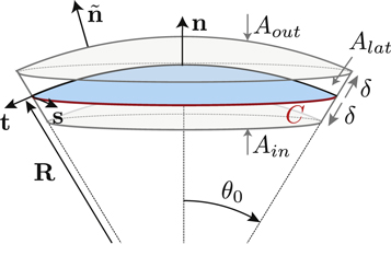
Figure B1. Geometry for the force balance. We consider a spherical cap of the droplet interface, with a box with constant distance δ to the interface inside and outside. The normal and tangential vectors  ,
,  and
and  of the interface are shown, as well as the normal vector
  of the box. The origin of the spherical coordinate system is the center of the sphere that describes the interfacial curvature, with radius
  , while
  gives the polar angle of the cap.
Download figure:
Standard image High-resolution imageNow let us consider the balance of the stress tensor equation (B.7) across the box, taking into account the curved geometry. The stress balance  can be written as

where α and β are Cartesian coordinates and  the (local, outward pointing) normal vector of the box-surface. We can split this in three terms,

where we used that the orientation of the normal vectors of the box coincides with the normal/tangential vector of the interface.
On the inner and outer areas Ain and Aout, the stress tensor presented in equation (B.8) with equilibrium stress tensor in equation (B.9) reduces to the form of the effective droplet model given after equation (6) in the main text, as the gradient terms are negligible for  . We now consider the limit of a sharp interface w → 0 with finite surface tension γ, and consider the case of a small box of thickness δ, which remains larger than the interfacial width. The components α = x, y of equation (B.23) vanish by symmetry. For α = z we find

where  are the stress tensor components of the effective model, equation (4), inside and outside the interface at
  . Integration over the lateral box surface Alat yields the last term,
  . We thus find that the mechanical equilibrium of a curved interface introduces a Laplace pressure 2γH,

We therefore recover the stress jump conditions of the effective droplet model, equation (6). Additionally, (B.25) together with (B.19) implies that the partial pressure needed to satisfy incompressibility is continuous across the interface,  .
.
B.3.3. Dynamics of the effective droplet model
We now consider the dynamics of a non-equilibrium system with a droplet. We show how the continuum model is related to the bulk equations and jump conditions of the effective droplet model. For this we consider a droplet with a interface that is thin compared to the dynamical length scales l±, so that we can describe the interface by local equilibrium. In the bulk phases we focus on the case where deviations from the equilibrium concentrations are small.
In the bulk phases, we expand the chemical potential equation (B.3) around the reference concentrations  . The gradient term −κ∇2c in the chemical potential is important within the interface, but can be ignored in the bulk phases, where the length-scales on which the concentration field varies are much larger than the interfacial width. Thus we can describe the chemical potential by

which is  for our specific free energy. With this simplification, equations (B.4) and (B.5) become the reaction-diffusion-convection equations (1) and (2) with diffusion constants
  or D± = Mb. Similarly we linearize the chemical reaction rate equation (B.6) in both phases. As we already chose a linear rate for the continuum model, we only need to relate the parameters k and ν with the constants k± and ν± of the effective model, with k± = k, ν+ = ν and ν− = kΔc − ν . Inserting the linearized chemical potential equation (B.26) into the equilibrium stress tensor (B.9) we find that momentum conservation in the bulk phases is given by the Stokes equation (4) with viscosities η± = η, where the pressure p is determined by the incompressibility condition ∂αvα = 0.
We consider the droplet interface to be in local equilibrium. We therefore obtain equation (8) for the jump of the concentration field in the effective model. The incompressibility condition ∂αvα = 0 implies  at a sharp interface, and we consider an interface without slip length, so that
  . We thus find equation (7) of the effective model. The normal stress balance in equation (6) is derived in B.3.2.
As a last point we need to find equation (10) for the interface movement. We consider the concentration change in a box of width δ around the interface, see figure B1. We consider a box enclosing a point  on the interface at the time t aligned with the normal and tangential directions of the interface at
  . The interface may move with normal movement
  , with
  and normal vector
  , while the box stays at a fixed position. The total change of material in the volume is given by

where V denotes the volume and A the area of the box. For small w and finite δ the concentration field c makes a jump from the surface Ain to Aout given by conditions (8) and (9) at  . Within each phase, we can express the field by the boundary values at the interface equation (B.21) and a linear expansion,

The chemical reaction is given in both phases by equation (B.6). For small δ and θ0, we find for the left-hand side of equation (B.27) that δc vanishes to lowest order and

where AR is the area of the droplet interface enclosed by the box. For a spherical cap,  . We further find that the source term due to the chemical reaction scales with the volume of the box, and thus vanishes for a small box,
  . The flux across the box can be expressed as

where  denotes the flux at
  inside/outside the droplet. We thus find the normal movement of the interface,

In the main text we use spherical coordinates centered at the droplet center. For a spherical droplet, the normal and radial movement would thus be the same. For a deformed droplet, we need to consider the relation between the normal interface movement,  and the radial movement
  . At fixed angles θ and ϕ, the interface movement is given by
  . Using
  , we find a relation between the radial and normal movement,
  . This relation, together with equation (B.31), yields the interfacial movement equation (10) presented in the main text.
We thus recover all dynamical equations of the effective droplet model from the continuum model based on irreversible thermodynamics. Note that the specific choice of the free energy leads to specific relations between parameters of the effective model such as D+ = D−. Our derivation shows the relation between both models in the case where the interface width w is small compared to the droplet size,  , and the chemical diffusion length,
  . Additionally, we focused on the case where the concentrations in the phases are similar to the concentrations in equilibrium and have small concentration gradients. These conditions are not valid in all systems. Most importantly, the chemical reactions can drive concentrations far away from the equilibrium phase concentrations
  . The resulting behaviors, such as the formation of new interfaces associated with instabilities of the spinodal decomposition regime, are not captured in the effective droplet model.
B.4. Comparison of the droplet dynamics in the continuum model and the effective model
Here we compare the analytical predictions of the effective model for the instability with numerical calculations of the continuous model for different values of the renormalized viscosity F. For this we numerically solved the dynamic equations of the continuous model starting with a droplet with a small initial deformation of mode l = 2. We fitted the dynamical behavior of the mode to an exponential function, with yields a numerical estimate for the eigenvalue μ2. In figure B2 the resulting eigenvalues are shown, together with the eigenvalue of corresponding parameters of the effective model. We find that the value of F for which droplet shapes become unstable is very similar to the value predicted by the effective model. The eigenvalues are qualitatively similar to the ones of the effective model, despite working in an a parameter regime where the interfacial width and the differences of concentration within a phase cannot be considered very small, so that the models are not necessarily comparable.

Figure B2. Growth of shape perturbations of the l = 2 mode for different normalized viscosities F = ηw/(γτ) for the continuous model (red crosses) and effective model (blue curve). The last data point (with arrow) corresponds to  . (Parameters: A = 8 × 10⁻³, = 0.2, η−/η+ = 1,
  , k+/k− = 1, ν−/(k−Δc) = 0.8.)
Download figure:
Standard image High-resolution image
To generate the data in the figure, we initialized droplets with a small shape perturbation for different values of F. All parameters and initial conditions were chosen as described in appendix B.2. We found that for  droplets divide, while they are stable for
  . For F = 10, the shape deformation was very slow, so that division was not seen in the time interval T/τ = 4000. For 10 < F < 100, as well as
  , we fitted radius and spherical harmonic deformation to the concentration field using equation (B.15). For short times, the droplet radius changes as the concentration field and droplet size go towards the stationary values. After that, the shape deformation grows until the droplet deforms so strongly that the fitting fails. By hand we chose intermediate time windows for the simulations where the size was stationary and the shape deformation small. In these windows we fitted the deformation amplitude (compare equation (B.15)) with an exponential function,
  with parameters A, B and eigenvalue μ2 to the l = 2 mode of the shape deformation.
Appendix C.: Estimation of parameters
Here we estimate the hydrodynamic parameter for two physical phase-separating systems to understand the importance of hydrodynamic flows on the droplet division in experimental systems. We discuss two cases, water–oil phase separation, and soft colloidal systems (such as protein-RNA phase-separation in cells). We have already estimated parameter values for both systems without the influence of hydrodynamic flows [39], where we found that droplet division should be possible for realistic values of chemical reaction rates in both systems, and that corresponding stationary radii would have sizes of a few micrometers. Here we estimate the value of the dimensionless viscosity F for water–oil and soft colloidal systems, and compare them to the analytical phase diagrams presented in figure 2.
To calculate the hydrodynamic parameter F for experimental systems, we need an estimation of the diffusion coefficient of the droplet material D+ outside the droplet, of the interfacial width w (which corresponds to length-scale w in the paper [39]), of the surface tension γ and of the viscosity η− inside the droplet. For water–oil systems, the interfacial width is of the order of  and the diffusion constant is D+ ≈ 10−9 m2 s–1. We can estimate the surface tension as γ ≈ 10−2 N m–1, and the viscosity η− ≈ 10−3 N s m–2 [54, 55]. With these values, we find F ≈ 0.1. In this case droplet division is strongly suppressed, see figure 2 of the main text. For soft colloidal systems, we estimate w ≈ 10 nm, D+ ≈ 10−10 m2 s–1 and γ ≈ 10−6 N m–1 [1, 54]. The value of F depends on the viscosity of the droplet. For values η− ≈ 10−3 N s m–2, F ≈ 10, and for η− ≈ 1–10 N s m–2, we have F ≈ 104. In both cases droplet division is possible, but more easy to achieve for larger F. We convert A* to the reaction rate ν− inside the droplet using the droplet concentration given in [39].
We can use equations (A.59) and (A.60) from the scaling analysis to estimate the instability of the concrete parameter examples discussed in [39] under the influence of hydrodynamic flows. In these scaling equations, the ratios η+/η− and D− β−/(D+ β+ ) enter the calculation of A* and * but we find that they do not lead to relevant changes in the results. The scaling analysis thus yields results very similar to the estimation using figure 2.