


Abstract
In a recent work devoted to the magnetism of Li2CuO2, Shu et al (2017 New J. Phys. 19, 023026) have proposed a 'simplified' unfrustrated microscopic model that differs considerably from the models refined through decades of prior work. We show that the proposed model is at odds with known experimental data, including the reported magnetic susceptibility χ(T) data up to 550 K. Using an 8th order high-temperature expansion for χ(T), we show that the experimental data for Li2CuO2 are consistent with the prior model derived from inelastic neutron scattering studies. We also establish the T-range of validity for a Curie–Weiss law for the real frustrated magnetic system. We argue that the knowledge of the long-range ordered magnetic structure for T < TN and of χ(T) in a restricted T-range provides insufficient information to extract all of the relevant couplings in frustrated magnets; the saturation field and INS data must also be used to determine several exchange couplings, including the weak but decisive frustrating antiferromagnetic interchain couplings.
Export citation and abstract BibTeX RIS

Original content from this work may be used under the terms of the Creative Commons Attribution 3.0 licence. Any further distribution of this work must maintain attribution to the author(s) and the title of the work, journal citation and DOI.
Li2CuO2 takes a special place among the still increasing family of frustrated chain compounds with edge-sharing CuO4 plaquettes and a ferromagnetic (FM) nearest neighbor (NN) inchain coupling J1 [1]. This unique position is due to its ideal planar CuO2 chain structure and its well-defined ordering characterized by a 3D Neél-type arrangement of adjacent chains whose magnetic moments are aligned ferromagnetically along the chains (b-axis). Li2CuO2 is well studied in both experiment and theory (see e.g. [2–11]) and serves nowadays as a reference system for more complex and structurally less ideal systems. In particular, it is accepted in the quantum magnetism community that the leading FM coupling is the NN inchain coupling J1. (J1 is also dominant but antiferromagnetic (AFM) in the special spin-Peierls case of CuGeO3 [12].) There is always also a finite frustrating AFM next-nearest neighbor (NNN) coupling J2 > 0, see figure 1, left. This inchain frustration is quantified by  . In the present case, and in that of the related Ca2Y2Cu5O10, there are only frustrating AFM interchain couplings (ICs) with adjacent chains shifted by half a lattice constant b. In this lattice structure there is no room for unfrustrated perpendicular IC. This AFM IC with NN and NNN components plays a decisive role in the stabilization of the FM alignment of the magnetic moments along the chain direction. Although weak at first glance, with eight NN and NNN it is nevertheless significant enough (by a factor of two) to prevent a competing non-collinear spiral type ordering in Li2CuO2 (with the frustration ratio α > 1/4), as often observed for other members of this family with unshifted chains [1]. All these well-established features were practically excluded by Shu et al (STL) [13], proposing instead (i) a very nonstandard unfrustrated model (dubbed hereafter as STL-model) with comparable couplings in all directions, and where the leading FM coupling is given by an unphysically large NNN FM IC Ja (denoted as J3 therein) perpendicular to the chains in the basal ab-plane (Ja = −103 K for stoichiometric and −90 K in the presence of O vacations in Li2CuO2−δ with δ = 0.16). (ii) The coupling between the NN chains, as derived from the inelastic neutron scattering (INS) data [6] and in qualitative accord with the results of LDA+U calculations [5], has been ignored and replaced ad hoc by an artificially large, 'effective' non-frustrated AFM IC
  (see the right of figure 9 in [13] with a 4-fold coordination) absent in real Li2CuO2.
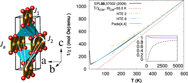
Figure 1. Left: the crystal structure of real Li2CuO2 and the main exchange couplings under debate (white lines: 1/4 of the skew AFM frustrating IC J5 and J6, between adjacent chains responsible for the FM inchain ordering but ignored in [13], similarly as the generic AFM NNN inchain coupling J2. There, the FM NN intrachain coupling J1 is underestimated by a factor of four (see table 1). Green line: the weak NNN IC  claimed to be dominant and FM by Shu et al [13]). Right: Main: the inverse spin susceptibility for a magnetic field along the a axis of Li2CuO2 (the sample that was used for INS studies, see figure 4 of [6]) fitted by the eight-order high-T expansion expression (10). Inset: convergence of the two pseudo-CW parameters to their high-T asymptotic values:
  (solid line),
  (dashed line).
Download figure:
Standard image High-resolution image
In the present Comment, we show that this parametrization is a direct consequence of an incorrect analysis of their susceptibility χ(T) data in addition to ignoring the highly dispersive magnon mode and its local softening observed by INS. We admit that the very question about an influence of O vacancies on the magnetic properties of Li2CuO2 raised by Shu et al [13] is interesting and should be studied; however, this must be done within a proper analysis based on a realistic phenomenological model reflecting the established large  values exceeding 200 K [6] and excludes a simple Curie–Weiss (CW) law below 1000 K. In this context we mention similar mistakes made in the literature, where even an artificial AFM ΘCW < 0 has been found [2, 14–16] prior to 2009, when the large value of J1 was not yet known.
Li2CuO2 is a frustrated quasi-1D system that has been well studied during the last decades. The first two rows of table 1 (see table 6 of [13]) provide the J's suggested by Shu et al from their qualitative simulation of the magnetic ordering and an analysis of the measured χ(T) for two samples with different O content. The main striking difference between these sets from all previous ones is the absence of both magnetic frustration and of the quasi-1D regime with a dominant J1 realized in all edge-sharing CuO2 chain compounds. Moreover, the proposed sets are evidently at odds with the results of two INS studies [6, 16]. The set derived from the INS in the bc plane [6] see the last row in table 1 (and table 6 of [13]) does explain the χ(T) data for T > TN, especially when supplemented by a weak AFM IC  to the a axis (in accord with the reported weakly dispersing magnon in that direction [16, 17]).
We consider the Heisenberg spin-Hamiltonian

where m enumerates the sites in the magnetic (Cu) lattice (see figures 1 and 9 of [13]), Jr is the interaction of a pair of spins  and
and  . Note the different notation with [16, 18, 19], where the same interaction is denoted −2Jr. The form of equation (1) implies positive (negative) signs for AFM (FM) couplings. Shu et al [13] use the same notation in tables 5 and 6, but use the wrong signs in equations (8) and (10). A small anisotropy of the couplings seems to be unimportant for the analysis of χ(T) and is ignored here. The magnetic field Hz is directed along the easy axis (i.e. the crystallographic a-axis in Li2CuO2). Finally, μB is the Bohr magneton and ga is the gyromagnetic ratio for this direction.
Shu et al use two approaches when analyzing χ(T) of Li2CuO2. First, they fit it in the range 250 K < T < 550 K using a CW-law

They then extract three effective couplings instead of six original ones by fitting χ (T) with an RPA-like expression derived for quasi-1D systems. Note that Shu et al give an obviously erroneous form in their equation (7) with the factor ![$[1-2({z}^{{\prime} }{J}^{{\prime} }+{z}^{{\prime\prime} }{J}^{{\prime\prime} })]$](https://content.cld.iop.org/journals/1367-2630/20/5/058001/revision1/njpaac159ieqn10.gif) , being a sum of the dimensionless value 1 and a value with the dimension of energy. No figure is shown for χ(T) fitted by their curve, so it is impossible to evaluate their fit, nor to estimate its quality and validity range. However, in [18] (reference 33 of their paper), the correct expression reads:
, being a sum of the dimensionless value 1 and a value with the dimension of energy. No figure is shown for χ(T) fitted by their curve, so it is impossible to evaluate their fit, nor to estimate its quality and validity range. However, in [18] (reference 33 of their paper), the correct expression reads:

where J = J1 is the inchain coupling and  = J3,
= J3,  are IC's with
  = 2,
= 2,  = 4 the corresponding numbers of neighbors (see figure 9(b) in [13] for a simplified structure, which differs from the real one, see figure 9(a) therein). In equation (3) we have accounted for the different notations of the exchange couplings between [13] (the same as ours) and [18]. Note that the quasi-1D regime assumed in equation (3) implies
  , which is obviously violated by the STL-model. We recall that a CW-law exactly reproduces the high-T behavior of the spin susceptibility of any system described by the Heisenberg Hamiltonian (1) with the CW temperature ΘCW

Equation (4) is the exact result of a high-T expansion (HTE) of the susceptibility [20] (see equation (27) of section IV.B in [21], see also [22], and references therein), which is valid for any Heisenberg system. As mentioned above, the expression for ΘCW given in equation (10) of [13] has a wrong sign. It gives positive (negative) contribution for AFM (FM) interactions in conflict with the physical meaning of ΘCW.
Now we show that χq1D also obeys a CW-law for large enough T. We recast equation (3) in the form

where C denotes the Curie constant, z = 2 is the inchain coordination number, and

The ΘCW = +14 K for the STL-model given by equation (4) should coincide with the value obtained by the CW fit presented in tables 3 and 4 of [13], provided the CW fit is justified for the chosen range of T. We stress that a value of ΘCW > 0 does not cause a divergence of χ (T) at T = ΘCW, in contrast to the erroneous claim of Shu et al in speculations after their equation (10). In general, a divergence of the susceptibility  means the emergence of a long-range order in a magnetic system characterized by a spontaneous magnetization m(Q0) for T < T0. A ferrimagnetic (FIM) and a FM ordering correspond to Q0 at the center of Brillouin zone (BZ) and to the uniform component of
  , respectively. Note that a FIM ordering and the divergence of
  may occur for systems with purely AFM couplings and negative ΘCW due to the geometry of the spin arrangement (see e.g. figure 4 of [23]). A
  corresponds to a helimagnetic or to an AFM ordering. Then, the uniform χ (T) remains finite at T0. An AFM ordering corresponds to Q0 located at the edge of the BZ. This is the case for the prior model of Li2CuO2, as well as for the STL-model. The range of validity of the CW-law for χq1D (equation (3)) is

As already noted, the approximate expression equation (3) is relevant for a quasi-1D system, where the inchain J's dominates. This is true also for the condition (7). Let us establish now a general condition for the applicability of a CW-law. For this aim it is convenient to use the inverted exact HTE [24] for spin-1/2 systems with equivalent sites

(see equations (5a), (5b) in [24]). Thus, a CW-law with ΘCW = −D1 is valid in the range

From this expression it is clear that for systems where both FM and AFM couplings are present, the CW behavior is valid at  . For the unfrustrated STL-model (the first row in table 1), the condition (9) reads
  K, while for the prior INS based model (the last row in table 1) it is
  K. One should also take into account that the convergence of the HTE is slow. To show that the exchange values determined from the INS are compatible with the χ (T) data, we reproduce in figure 1 the data measured on the same sample (i.e. with the same O content) used for the INS studies (see figure 4 of [6]). We have fitted the data in the range 340 < T < 380 K with the expression

where χ8(T) is the eighth-order HTE obtained by the method and programs published in [25]16
, and NA is Avogadro's number. The HTE program of [25] we have used here can only treat systems with four different exchange couplings only, so we decided to adopt one effective coupling in the a direction Ja = J3 + 2J4. Only one parameter ga was adjusted during the fit despite the small background susceptibility χ0 which was set to zero for the sake of simplicity and its insensitivity to our fit. The [4,4]-Padé approximant for the HTE fits the data well down to T ∼ 20 K with the reasonable value ga = 2.34. The inset shows  and
and  , the two parameters of the pseudo-CW-law (see figure 4 of [6]), which is given by a tangent to the 1/χ(T) curve at a given T. The pseudo-Curie 'constant'
  exceeds its asymptotic value for all T. Hence, it cannot be used to extract the number of spins in the system. The C from a more elaborate HTE is much better suited for this aim. For example, a clear crossover between a CW (without any divergence at ΘCW = +39 K) and a pseudo-CW regimes has been observed recently near 150 K for CuAs2O4, see figures 8 and 9 in [26].
We note that the difficulties encountered at intermediate T when avoiding the use of a HTE as demonstrated above can be circumvented by applying a strong magnetic field (up to saturation at Hs where the AFM IC is suppressed). At very low-T and in the isotropic limit, one has a very simple but useful relation

The quantities on the rhs can be deduced from the INS data [6, 17]. Indeed, with J1 = −230 K, α = 0.326, Hs = 55.4 T for  , gb = 2.047 [27], and Ja ≈ 8 K, we arrive nearly at the same ΘCW = 54 K as in the HTE analysis of χ(T). For collinear systems, Hs is related to the inter-sublattice couplings (see equation (1) in [27], valid at T = 0)

where NIC = 8 is the number of nearest IC neighbors, JIC = J6, and  = J5. Equation (12) gives
  = 9.5 K, close to the value from our model. Conversely, equation (12) gives
  T for the STL-model, even for the unrealistic value ga = 2.546 (table 3 of [13]), which much exceeds the observed 55 T. Thus, Shu et al's
  value is at odds with the high-field data reported in 2011 [27]. Shu et al have also ignored the T-dependence of the RIXS (resonant inelastic x-ray spectroscopy) spectra of Li2CuO2 reported in 2013 [7], which were explained within a pd-model consistent with the INS data. The detection of an intrachain Zhang–Rice singlet exciton at T > TN and significant increase of its weight at 300 K evidence the increase of AFM correlations in the chain and cannot be explained without a frustrating AFM intrachain coupling J2.
Next, we remind the reader of some microscopic insights into the magnitude of the exchange couplings for Li2CuO2. Empirically, a dominant FM J1 [6, 17] and the minor role of Ja [6, 16, 17] follow directly from the observed strong (weak) dispersion of the magnons along the b (a)-axis, respectively. Microscopically, the large value of J1 as compared with −100 K suggested in [28] is a consequence of an enlarged direct FM exchange Kpd between two holes on Cu and O sites within a CuO4 plaquette and the non-negligible Hunds' coupling between two holes in different O 2px and 2py orbitals in edge-sharing CuO2 chain compounds. The former is well-known from quantum chemistry studies (QCS) of corner-sharing 2D cuprates having similar CuO4 plaquettes with Kpd,π ≈ −180 meV for Φ = 180° Cu–O–Cu bond angles [29]. Now we confirm similar values of the two Kpd interactons in Li2CuO2 using QCS [30], which yielded for Φ ≈ 90o:  , (ignoring a weak crystal field splitting of the two O onsite energies). Thus, our two
  values being naturally slightly different are more than twice as large as −50 meV for both direct FM couplings ad hoc adopted in [12, 28, 31] in the absence of QCS calculations for Li2CuO2 and CuGeO3 [12, 31] 20 years ago. Concerning Ja, QCS yield a small direct FM dd contribution ≈−1 K, while our DFT-derived Wannier-functions point to a tiny AFM value of about 5 K. A more direct calculation within the LDA+U scheme for large supercells is in preparation. Anyhow, even with possible error bars of the DFT and QCS calculations, a value of Ja exceeding ±10 K is not expected. Hence, a much larger Ja ≈ −103 K as suggested by Shu et al is either an artifact from the constructed 'simplified' non-frustrated STL-model and/or a consequence of the improperly analyzed χ(T)-data, as explained above.
Thus, we have shown that the 'effective' unfrustrated STL-model proposed by Shu et al together with its doubtful analysis of χ(T) are at odds with our current understanding of real Li2CuO2 and will only confuse readers. It may, however, be of some academic interest to illustrate the crucial effect of intra- and IC frustrations evidenced by a recent INS study. In case of finite NNN exchange J2 with α > αc = 1/4, as evidenced by the minimum of the magnon dispersion near the 1D propagation vector, there would be an inphase or antiphase ordering of non-collinear spirals for FM (AFM) perpendicular IC  [32]. Such a situation would also be realized for an STL-model corrected by α > αc, in sharp contrast to the observed collinear magnetic moments aligned ferromagneticaly along the chain direction with weak quantum effects. In this context, we note that we know of no example of a frustrated model that can be replaced comprehensively by a non-frustrated effective model as Shu et al have tried to do. We admit that some selected special properties like the long-wave susceptibility at q = 0, if treated properly by a HTE, could be approximated this way. But quantities (e.g. χ(q, ω)) with the q-wave vector in the vicinity of the 1D 'propagation vector' defined by the maximum of the 1D magnetic structure factor S(q, 0) certainly do not belong to them. This is clearly evidenced by the magnon minimum (soft spin excitation above about 2.5 meV, only, from the ground state) as seen in the INS [6] reflecting the vicinity to a critical point. Thus, the low-energy dynamics of both models are different since the microscopic mechanisms and the stability of the FM inchain ordering are completely distinct for these two approaches.
We hope that our detailed discussion of χ(T) at intermediate T is of interest to a broader readership. We have drawn attention to the available HTE computer codes. Thereby we stress that the usual smooth behavior of χ (T) does not allow one to deduce multiple exchange parameters, especially if the maximum and the submaximum regions at low-T are not involved in the fit. Other thermodynamic quantities such as the saturation field, magnetization, specific heat, and INS data must be included. What can and must be done when dealing with χ(T), is to check the compatibility of already existing derived or proposed parameter sets with experimental χ (T) data. The model proposed by Shu et al has not passed our χ-check. Their argument against our FM ΘCW ≈ 50 K [6] due to a seemingly 'incomplete selection of fitting parameters' is obsolete since a weak Ja value has been included in our refined analysis resulting now in ΘSW ≈ 55 K. The stressed seemingly divergence of χ(T) at T = ΘCW ≈ 50 K of our frustrated set does not reflect 'an inconsistency' of our approach as claimed by Shu et al. Rather, it provides just a proof and documents only that the authors did not consider the restricted regions of validity for any CW-law approaching even intermediate and of course lower T! In this context, we mention that, if the authors would have inserted their own correct sign values for ΘCW > 0 derived from its definition by equation (4) (see table 1), they would be confronted themselves with the same pseudo-problem they have tried to accuse us! Their referring to the work [33]17 as a 'first principle density functional theory (DFT)' explanation for why a spiral ordering is missing, is somewhat misleading. There the relative weak frustrating AFM IC's and the related and observed [6] dynamical spiral fluctuations were ignored but Xiang et al [32] arrived nevertheless at a non-negligible finite J2 value above αc = 1/4, in qualitative accord with the INS data [6]. To the best of our knowledge, there is no edge-sharing chain cuprate with a vanishing J2 and a finite frustrating AFM value is considered to be generic for the whole family. There is no reason to prescribe a seemingly vanishing J2 value to the presence of a significant level of O vacancies in high-quality samples. The INS [6, 17] and RIXS data [10] provide clear evidence for a skew AFM IC with no need for a speculative and exotic 'order from disorder' scenario.
Table 1.
Exchange sets proposed for the 'effective' unfrustrated STL-model and our frustrated one for real Li2CuO2 in the notations of [13], see figures 9(a) and (b), respectively, therein. Ja = J[1, 0, 0], J5 = ![$J[\tfrac{1}{2},\tfrac{1}{2},\tfrac{1}{2}]$](https://content.cld.iop.org/journals/1367-2630/20/5/058001/revision1/njpaac159ieqn34.gif) , and J6 =
, and J6 = ![$J[\tfrac{1}{2},\tfrac{3}{2},\tfrac{1}{2}]$](https://content.cld.iop.org/journals/1367-2630/20/5/058001/revision1/njpaac159ieqn35.gif) in crystalographic notations.
in crystalographic notations.
| Ji/kB (K) | J1 | J2 |

|
J4 | J5 |

|
J6 | ΘCW(K) |
|---|---|---|---|---|---|---|---|---|
| zi | 2 | 2 | 2 | 4 | 8 | 4 | 8 | |
| [13](δ ∼ 0.16) | −61 | 0 | −90 | 0 | — | 62 | 0 | 14 |
| [13] (δ ∼ 0) | −65 | 0 | −103 | 0 | — | 71.2 | 0 | 13 |
| [6] | −228 | 76 | — | — | 0 | — | 9.04 |

|
| [17], present | −230 | 75 | 4.8 | 1.6 | 0 | — | 9 | 56 |
To summarize, the frustrated model for Li2CuO2, refined by the INS data [6, 16, 17] (see the last row in table 1), our DFT and five-band pd-Hubbard model calculations [6], are consistent with the experimental data, including the χ (T) [6], the field dependent magnetization, the saturation field value [27], and the T-dependent RIXS spectra [7]. This is in contrast to the SLT-model, which does not account for these data. Due to lacking space a critical discussion of the O vacancy scenario and the related Cu 4p hole bonding scenario by Shu et al instead of the correlated Cu 3d covalent electron picture must be considered elsewhere. We mention here only that the main reason for disorder in Ca2Y2Cu5O10 is likely not the presence of O vacancies, as stated by Shu et al, but the intrinsic misfit with the Ca2+Y3+-chains that surround and distort the CuO2 chains [34–36]. Based on this complex structure there are no hints pointing to O vacancies.
Acknowledgments
ROK thanks the Heidelberg University for hospitality. Also the project III-8-16 of the NASc of the Ukraine and the NATO project SfP 984735 are acknowledged. SN thanks the SFB 1143 of the DFG for financial support. MM acknowledges the support by the Scientific User Facilities Division, Office of Basic Energy Sciences, US DOE. We appreciate discussions with A. Tsirlin, B Büchner, V Grinenko, and K Wörner. The publication of this article was funded by the Open Access Fund of the Leibniz Association.
Footnotes
- 16
The corresponding HTE package used in [25] we have employed obtaining the results shown here, too. It is available at www.uni-magdeburg.de/jschulen/HTE/
- 17
Here, ignoring any IC due to its seemingly weakness, the origin of the FM inchain ordering instead of the expected spiral ordering for α > 1/4 the final TN has been attributed to an 'order from disorder'-transition.