Noise resistant quantum control using dynamical invariants

A major obstacle to manipulate quantum systems and develop quantum technologies is the unavoidable presence of noise. There are different types of noise sources that disturb control protocols, including noise induced by the environment, noise caused from interaction with the measurement apparatus, or errors in the implementation of the control protocol. Different approaches proposed to suppress or mitigate the effects of noise include (for a recent review see [1]): the use of decoherence-free subspaces which are immune to noise [2], correction of errors using quantum feedback controls [3], performing sudden interactions on the system on timescales for which the noise only slightly interferes with the process such as in dynamical decoupling [4], and applying shortcuts to adiabaticity (STA) [5, 6]. The noise has also been proposed as a resource to achieve the desired control in specific processes [7–9].

A large family of control protocols are based on adiabatic following of instantaneous eigenstates of a time dependent Hamiltonian by smoothly and slowly changing control parameters. These methods are widespread as they are in principle robust against control imperfections. However, they are also prone to suffer the effects of noise due to long operation times. As a result the fidelity of the final state with respect to the target state is reduced [1, 10].

STA are control methods to derive protocols which reach fidelities of slow adiabatic processes in significantly shorter times. STA have been applied in a wide variety of fields including quantum computation [11–14], cooling [5, 15], quantum transport [16, 17], quantum state preparation [18–21], cold atoms manipulation [22–28], many-body state engineering [29–32] and polyatomic molecules control [33], design of optical devices [34, 35] and linear chains [36], or mechanical engineering [37, 38].

STA provide a strategy to combat the effects of noise thanks to two different mechanisms: (i) In principle faster than adiabatic processes are desirable to avoid pervasive, long interactions with the environment. In practice the fidelities may present maxima at specific times [8], and STA can be set for these optimally short process times. Many studies have tested the achieved robustness with master equations including the noise, see e.g. [39, 40]; (ii) in addition, the parameter paths leading to STA are typically not unique, so this freedom may be used to choose the most robust ones with respect to specific perturbations, noise or control imperfections. This optimization has been performed so far by minimizing the excitation energy or maximizing the fidelity in perturbative schemes, e.g. in two-level systems (TLSs) [41–44] or for ion transport [45], using decoherence free subspaces [46, 47], super-operator [48] and non-Hermitian invariants [49], and effective Hamiltonians [50].

In this work we introduce an alternative systematic method for smooth control under the influence of noise which is applicable for both adiabatic and nonadiabatic time scales. The technique proposed intends to go beyond the perturbative regime and can be applied to the strong noise regime [51]. The central idea is to inverse engineer the noiseless Hamiltonian by designing its dynamical invariants (i.e., the dynamics of the noiseless system) such that the noise has a minimal effect. The control functions to be minimized are state independent, and measure the deviation of the actual invariant, i.e., the one for the full dynamics including noise, from the noiseless invariant. This technique does not require one to solve the full dynamics iteratively as is often done in optimal control methods [52, 53]. This property makes the method appealing and simple for implementation. Furthermore, it is not restricted to very fast operations, where typically very short control time is limited by experimental constraints.

The dynamics of the system including the dissipative term resulting from the noise takes the form (for ${\hslash }=1$)

$$\begin{eqnarray}&&\displaystyle \frac{{\rm{d}}\hat{\rho }}{{\rm{d}}{t}}=-{\rm{i}}[\hat{H}(t),\hat{\rho }]+{ \mathcal L }\hat{\rho },\end{eqnarray} \tag{ 1 }$$

where

$$\begin{eqnarray}&&{ \mathcal L }\hat{\rho }=-\displaystyle \sum _{k}{\eta }_{k}[{\hat{X}}_{k}(t),[{\hat{X}}_{k}(t),\hat{\rho }]]\quad {\text{}}{\rm{with}}\quad {\eta }_{k}\gt 0.\end{eqnarray} \tag{ 2 }$$

Here $\hat{H}(t)$ is the total Hamiltonian of the system including the control Hamiltonian and the noise term given by equation (2). The ${\hat{X}}_{k}(t)$ represent Hermitian operators acting on the Hilbert space of the system and can be explicitly time dependent. The pre-factors ${\eta }_{k}$ are scaling factors representing the strength of the noise and may have different dimension depending on ${\hat{X}}_{k}(t)$. The sum over k includes the possibility of independent types of noise simultaneously affecting the dynamics. This equation was derived in different contexts, including the singular coupling limit [54], phase noise [55], action noise [8], amplitude noise [56], quantum noise from monitoring weakly the quadrature of the system [3, 57], Gaussian noise and Poisson noise for SU(2) algebra [58, 59], and more [60–62].

In section 2 we present the main results of this work. First we construct the dynamical invariant method in the density operator formalism which can also be then applied to the study of noise and naturally extend the treatment from pure states to general mixed states. We derive two measures to quantify the effect of noise introducing constraints on the noiseless dynamical invariant. In section 3 we study the example of the TLS with single and multiple noise terms in the dynamics. Section 4 studies the control of thermal and coherent states of the harmonic oscillator. We conclude with a discussion and outlook on future work in section 5, plus some technical appendices.

2.1. Dynamical invariant for unitary dynamics

We refer the reader who is unfamiliar with the dynamical invariant method to appendix A where we present the method in the wave function formalism.

For noiseless, unitary dynamics, the evolution of the density operator is described by

$$\begin{eqnarray}&&\displaystyle \frac{{\rm{d}}\hat{\rho }}{{\rm{d}}{t}}=-{\rm{i}}[\hat{H}(t),\hat{\rho }].\end{eqnarray} \tag{ 3 }$$

A dynamical invariant satisfies the equation [63]

$$\begin{eqnarray}&&\displaystyle \frac{{\rm{d}}\hat{I}}{{\rm{d}}{t}}\equiv {\rm{i}}\displaystyle \frac{\partial \hat{I}(t)}{\partial t}-[\hat{H}(t),\hat{I}(t)]=0,\end{eqnarray} \tag{ 4 }$$

and therefore its expectation values for an arbitrary solution of equation (3) do not depend on time. It can be expressed in diagonal form,

$$\begin{eqnarray}&&\hat{I}(t)=\displaystyle \sum _{k}{\lambda }_{k}| {\phi }_{k}\rangle \langle {\phi }_{k}| .\end{eqnarray} \tag{ 5 }$$

Here λ_k are the real time independent eigenvalues and $| {\phi }_{k}\rangle \equiv | {\phi }_{k}(t)\rangle$ are the time dependent eigenvectors of the invariant. In this basis, the density matrix elements ${\rho }_{{lk}}\equiv \langle {\phi }_{l}| \hat{\rho }(t)| {\phi }_{k}\rangle$ can be calculated from

$$\begin{eqnarray}&&{\dot{\rho }}_{{lk}}={\rm{i}}\left(\langle {\phi }_{l}| {\rm{i}}\displaystyle \frac{\partial }{\partial t}-\hat{H}(t)| {\phi }_{l}\rangle -\langle {\phi }_{k}| {\rm{i}}\displaystyle \frac{\partial }{\partial t}-\hat{H}(t)| {\phi }_{k}\rangle \right){\rho }_{{lk}},\end{eqnarray} \tag{ 6 }$$

where the dot represents the time derivative. The off diagonal terms of the density matrix depend on the difference of time derivatives of two Lewis–Riesenfeld phases (compare with equation (A.5)), while the populations remain constant with time [63]. A system initialized in an eigenstate of the invariant evolves in this same eigenstate without transitions, imposing $[\hat{I}(0),\hat{H}(0)]=[\hat{I}({t}_{f}),\hat{H}({t}_{f})]=0$ we ensure that the system starts and ends in an energy eigenstate of $\hat{H}$ without unwanted excitations. The state transfer is designed by choosing $\hat{I}(t)$ and then determining $\hat{H}(t)$. (More details in appendix A.)

2.2. Dynamical invariant under the influence of noise

We now consider the influence of equation (2) on the control process. In order to demonstrate the effect of noise we consider a single operator $\hat{X}\equiv {\hat{X}}_{1}(t)$ and η ≡ η₁. In a later example, we will also consider the case for simultaneous noise sources. The dynamics for an arbitrary observable $\hat{A}$ including the noise effect in the Heisenberg representation reads

$$\begin{eqnarray}&&\displaystyle \frac{{\rm{d}}\hat{A}}{{\rm{d}}{t}}=\displaystyle \frac{\partial \hat{A}}{\partial t}+{\rm{i}}[\hat{H},\hat{A}]-\eta [\hat{X},[\hat{X},\hat{A}]].\end{eqnarray} \tag{ 7 }$$

Assuming the structure of the invariant (5) for the unitary dynamics we insert it in equation (7) to account for the noise. The eigenvalues of the invariant λ_l are now no longer constant in time and evolve according to

$$\begin{eqnarray}&&{\dot{\lambda }}_{l}=2\eta \left({\lambda }_{l}\langle {\phi }_{l}| {\hat{X}}^{2}| {\phi }_{l}\rangle -\displaystyle \sum _{k}{\lambda }_{k}| \langle {\phi }_{k}| \hat{X}| {\phi }_{l}\rangle {| }^{2}\right).\end{eqnarray} \tag{ 8 }$$

Note that if $\{| {\phi }_{k}\rangle \}$ are eigenstates of $\hat{X}$ then ${\dot{\lambda }}_{l}=0$ as required in the unitary noiseless method. In this case the invariant is not affected by the noise. Although the requirement for $\hat{I}$ and $\hat{X}$ having common eigenstates cannot generally be achieved for all times during the process, the effect of noise can be significantly reduced by constructing the Hamiltonian from an invariant which shares common eigenvectors with those of $\hat{X}$ during most of the process. Since at final time we impose that the invariant and the Hamiltonian share common eigenstates, protecting the invariant from the noise will drive the system to the desired target state.

To express the density matrix elements, equation (6) is now modified by adding to the rhs the additional term ${\dot{\rho }}_{{lk}}^{d}\equiv \langle {\phi }_{l}| { \mathcal L }\hat{\rho }| {\phi }_{k}\rangle$ which accounts for dissipation and decoherence resulting from the noise term and is given by

$$\begin{eqnarray}&&{\dot{\rho }}_{{lk}}^{d}=-\eta \left[\displaystyle \sum _{n}({\rho }_{{nk}}\langle {\phi }_{l}| {\hat{X}}^{2}| {\phi }_{n}\rangle +{\rho }_{{ln}}\langle {\phi }_{n}| {\hat{X}}^{2}| {\phi }_{k}\rangle )-2\displaystyle \sum _{{nm}}{\rho }_{{nm}}\langle {\phi }_{l}| \hat{X}| {\phi }_{n}\rangle \langle {\phi }_{m}| \hat{X}| {\phi }_{k}\rangle \right].\end{eqnarray} \tag{ 9 }$$

In the limit that $\hat{I}$ and $\hat{X}$ share common eigenstates the contribution due to noise to the change in population and the off diagonal terms is

$$\begin{eqnarray}{\dot{\rho }}_{{kk}}^{d} & \to & 0\\ {\dot{\rho }}_{{lk}}^{d} & \to & -\eta {({x}_{l}-{x}_{k})}^{2}{\rho }_{{lk}},\end{eqnarray} \tag{ 10 }$$

where $\{{x}_{k}\}$ are the eigenvalues of $\hat{X}$. Note that in this limit the decay of the populations in the invariant eigenbasis is suppressed, however, a decay of the coherences is still present, although it can be minimized for sufficiently fast processes.

The strategy proposed here relies on the ample freedom provided by STA. By adding constraints on the unitary invariant we can design a control Hamiltonian that optimizes the fidelity under the influence of the noise.

To identify the amount of overlap between the two bases sets of $\hat{I}$ and $\hat{X}$ we define the overlap matrix S with the entries

$$\begin{eqnarray}&&{S}_{{ij}}(t)=\langle {\phi }_{i}| {\psi }_{j}\rangle .\end{eqnarray} \tag{ 11 }$$

Here $\{| {\psi }_{j}\rangle \}$ are the eigenvectors of $\hat{X}$. The sum of the overlap matrix can be bounded by: $n\leqslant {\sum }_{{ij}}^{n}| {S}_{{ij}}| \lt {n}^{2}$, where n is the dimension of the space. The upper bound is not tight, and obtaining a tight bound, typically, becomes a difficult optimization problem for high dimension. However, we are only interested in minimizing S. In the scenario of n = 2, the tight upper bound is given by $2\sqrt{2}$. Next, we define the measure for the overlap along the process as the time average of the distance between the overlap matrix and its minimal value.

$$\begin{eqnarray}&&{ \mathcal O }:= \displaystyle \frac{1}{{t}_{f}}{\int }_{0}^{{t}_{f}}\left(\displaystyle \sum _{{ij}}^{n}| {S}_{{ij}}| -n\right){\rm{d}}{t}.\end{eqnarray} \tag{ 12 }$$

The measure ${ \mathcal O }$ is zero if and only if the eigenbasis of $\hat{X}$ and $\hat{I}$ are identical. A different measure which stems from similar considerations and in some cases can be easier to compute is

$$\begin{eqnarray}&&{ \mathcal A }:= {z}^{-1}{\int }_{0}^{{t}_{f}}\parallel [\hat{X}(t),\hat{I}(t)]\parallel {\rm{d}}{\rm{t}}=\displaystyle \frac{{\int }_{0}^{{t}_{f}}{\rm{d}}{\rm{t}}\sqrt{2{\rm{tr}}({\hat{I}}^{2}{\hat{X}}^{2})-2{\rm{tr}}(\hat{I}\hat{X}\hat{I}\hat{X})}}{2{\int }_{0}^{{t}_{f}}{\rm{d}}{\rm{t}}\sqrt{{\rm{tr}}({\hat{I}}^{2}{\hat{X}}^{2})}}.\end{eqnarray} \tag{ 13 }$$

In the above expressions we use the Frobenius norm defined as $\parallel { \mathcal M }\parallel \equiv \sqrt{\mathrm{tr}({ \mathcal M }{{ \mathcal M }}^{\dagger })}$. The normalization factor $z=2{\int }_{0}^{{t}_{f}}\parallel \hat{X}(t)\hat{I}(t)\parallel {\rm{d}}{t}$ guarantees that ${ \mathcal A }$ is dimensionless and equal or smaller than 1 (this is an immediate consequence of the sub-additivity of the Frobenius norm). The measure ${ \mathcal A }$ is zero if and only if $\hat{X}$ and $\hat{I}$ commute at all times during the process $\hat{I}\hat{X}=\hat{X}\hat{I}$, and takes the maximal value ${ \mathcal A }=1$ when $\hat{I}\hat{X}=-\hat{X}\hat{I}$. For unbounded operators extra care is needed. The norm should be calculated on a finite domain or using other techniques as will be demonstrated in a later section.

In order to improve the fidelity of the evolved state with respect to the target by minimizing the effect of noise, the controls that drive the system are inverse engineered through the invariant $\hat{I}(t)$ of the unitary dynamics subject to the minimization of the measures ${ \mathcal O }$ or ${ \mathcal A }$.

As a first example we consider the control problem of a full population inversion in a TLS [18, 64–67]. The Hamiltonian takes the form:

$$\begin{eqnarray}&&\hat{H}(t)=\displaystyle \frac{{\rm{\Delta }}(t)}{2}{\hat{\sigma }}_{z}+\displaystyle \frac{{\rm{\Omega }}(t)}{2}{\hat{\sigma }}_{x},\end{eqnarray} \tag{ 14 }$$

where Δ(t) and Ω(t) are real, time-dependent functions resulting from an interaction with some external field, and ${\hat{\sigma }}_{z}$ and ${\hat{\sigma }}_{x}$ are the Pauli matrices. Initially the system is set to the ground state, ${\hat{\rho }}_{0}=| 0\rangle \langle 0|$, with the initial Hamiltonian corresponding to ${\rm{\Delta }}(0)={{\rm{\Delta }}}_{0}$ and ${\rm{\Omega }}(0)=0$. The desired target state ${\hat{\rho }}_{{\rm{tar}}}=| 1\rangle \langle 1|$ corresponds to the ground state of the final Hamiltonian Δ(t_f) = −Δ₀ and Ω(t_f) = 0. To evaluate the success of the control protocol we will use the fidelity

$$\begin{eqnarray}&&{ \mathcal F }:= \mathrm{tr}\sqrt{\sqrt{\hat{\rho }({t}_{f})}{\hat{\rho }}_{{\rm{tar}}}\sqrt{\hat{\rho }({t}_{f})}},\end{eqnarray} \tag{ 15 }$$

that measures the overlap between the final state and the target state ${\hat{\rho }}_{{\rm{tar}}}$. To connect the states $\hat{\rho }(0)$ and ${\hat{\rho }}_{{\rm{tar}}}$ we engineer the controls Δ(t) and Ω(t) from the dynamical invariant. Associated with the Hamiltonian (14) there is a dynamical invariant expressed as (see appendix B),

$$\begin{eqnarray}&&\hat{I}(t)=\sqrt{{{\rm{\Delta }}}^{2}(0)+{{\rm{\Omega }}}^{2}(0)}(\cos (G){\hat{\sigma }}_{z}+\sin (G)\cos (B){\hat{\sigma }}_{x}-\sin (B){\hat{\sigma }}_{y}),\end{eqnarray} \tag{ 16 }$$

where G ≡ G(t) and B ≡ B(t) are auxiliary real time dependent functions of the invariant obeying

$$\begin{eqnarray}&&{\rm{\Delta }}=-\dot{B}+\displaystyle \frac{\dot{G}}{\tan (G)\tan (B)},\quad {\rm{\Omega }}=\displaystyle \frac{\dot{G}}{\sin (B)}.\end{eqnarray} \tag{ 17 }$$

The frictionless conditions $[\hat{H}({t}_{b}),\hat{I}({t}_{b})]=0$ at t_b = 0, t_f impose at the boundary times fix $G(0)=\pi ,G({t}_{f})=0,\dot{G}({t}_{b})=0$, leaving B(t_b) and $\dot{B}({t}_{b})$ as free parameters (appendix B). At intermediate times these two functions are totally free. In particular interpolating $G(t)={\sum }_{i=0}^{3}{g}_{i}{t}^{i}$ and $B(t)={\sum }_{i=0}^{3}{b}_{i}{t}^{i}$ by polynomials with at least the same degree as the number of boundary conditions lets us deduce from equation (17) the desired controls Δ(t) and Ω(t). However, extra coefficients can be added to the interpolation, for example, $G(t)={\sum }_{i=0}^{4}{g}_{i}{t}^{i}$. Here g₄ can be used to also control the values of the measures ${ \mathcal O }$ or ${ \mathcal A }$.

3.1. Single noise source

We first consider amplitude noise of the form ${\hat{X}}_{1}\equiv {\hat{\sigma }}_{z}$ and η₁ ≡ η_z. For this particular type of noise the measure ${ \mathcal O }$ is given explicitly by

$$\begin{eqnarray}&&{{ \mathcal O }}_{z}=\displaystyle \frac{1}{{t}_{f}}{\int }_{0}^{{t}_{f}}2\left(\left|\sin \left(\displaystyle \frac{G}{2}\right)\right|+\left|\cos \left(\displaystyle \frac{G}{2}\right)\right|-1\right){\rm{d}}{t},\end{eqnarray} \tag{ 18 }$$

which is independent of the free function B of the invariant. It takes its minimal value ${{ \mathcal O }}_{z}\to 0$ when $G(t)\to n\pi$ with $n\in {\mathbb{Z}}$ and the maximal $2\sqrt{2}-2$ when $G(t)\to \pi /2+n\pi$. Similarly we can write explicitly (13) after some simple algebra:

$$\begin{eqnarray}&&{{ \mathcal A }}_{z}=\displaystyle \frac{{\int }_{0}^{{t}_{f}}{\rm{d}}{t}| \sin (G)| }{{t}_{f}}.\end{eqnarray} \tag{ 19 }$$

As for the measure ${{ \mathcal O }}_{z}$ the minimal value ${{ \mathcal A }}_{z}\to 0$ occurs when $G\to n\pi$ and ${{ \mathcal A }}_{z}\to 1$ for $G\to \pi /2+n\pi$.

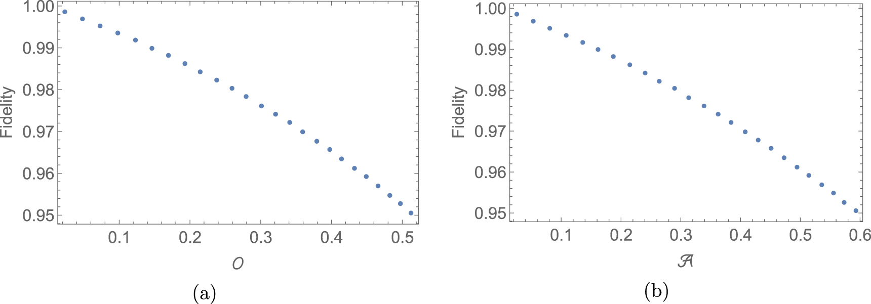
In figure 1 we plot the fidelity as function of the measures ${{ \mathcal O }}_{z}$ and ${{ \mathcal A }}_{z}$ for a given final time t_f for the full population inversion problem. Both measures show a similar behavior, when ${{ \mathcal O }}_{z}\to 0$ and ${{ \mathcal A }}_{z}\to 0$ the fidelity is improved significantly and monotonically decreasing as ${{ \mathcal O }}_{z}$ and ${{ \mathcal A }}_{z}$ increase. Thus, by adding constraints on these measures when constructing the invariant we obtain a control field which minimizes the effect of the noise. When the dynamics is subject to noise from a single source, i.e., a single ${\hat{X}}_{1}$, a control protocol which leads to fidelity ≃1 can be found. Generally, when the dynamics is subject to several independent sources of noise, ${\hat{X}}_{j}$, obtaining fidelity ≃1 is not guaranteed. Nevertheless, the influence of the overall noise can still be minimized and the final fidelity is improved.

Zoom In Zoom Out Reset image size

3.2. Multiple noise sources

When multiple noise terms (different ${\hat{X}}_{j}$) are present in the dynamics, the measures ${{ \mathcal O }}_{j}$ or ${{ \mathcal A }}_{j}$ cannot always be minimized simultaneously. In the next example we study the worst case scenario where the two noise terms have mutually unbiased bases [68]. In this case minimization of one of the noise terms will lead to maximization of the other. In particular we consider amplitude noise both in the ${\hat{\sigma }}_{z}$ and ${\hat{\sigma }}_{x}$ fields, i.e., ${\hat{X}}_{1}={\hat{\sigma }}_{z},{\eta }_{1}={\eta }_{z}$ and ${\hat{X}}_{2}={\hat{\sigma }}_{x},{\eta }_{2}={\eta }_{x}$. For the TLS we employ ${{ \mathcal O }}_{z(x)}$ to quantify the effect of the noise in the dynamics. As for ${{ \mathcal O }}_{z}$ we can write explicitly ${{ \mathcal O }}_{x}$ as

$$\begin{eqnarray}&&{{ \mathcal O }}_{x}=\displaystyle \frac{1}{{t}_{f}}{\int }_{0}^{{t}_{f}}2\left(\sqrt{\displaystyle \frac{1-\cos (B)\sin (G)}{2}}+\sqrt{\displaystyle \frac{1+\cos (B)\sin (G)}{2}}-1\right){\rm{d}}{t}.\end{eqnarray} \tag{ 20 }$$

By examining the integrands of equations (18) and (20) we observe that (i) when $G(t)\to n\pi$, then ${{ \mathcal O }}_{z}\to 0$ and ${{ \mathcal O }}_{x}$ approach its maximal value $2\sqrt{2}-2$, independently of B(t). The other extreme limit is obtained (ii) when $G(t)\to \pi /2+n\pi$ and $B(t)\to n\pi$, then, ${{ \mathcal O }}_{z}\to 2\sqrt{2}-2$ and ${{ \mathcal O }}_{x}\to 0$. For multiple noise terms we suggest to minimize the average $\bar{{ \mathcal O }}$ of the single noise measures weighted according to their relative strength. In the example above this average reads,

$$\begin{eqnarray}&&\bar{{ \mathcal O }}=\displaystyle \frac{{\eta }_{z}}{{\eta }_{z}+{\eta }_{x}}{{ \mathcal O }}_{z}+\displaystyle \frac{{\eta }_{x}}{{\eta }_{z}+{\eta }_{x}}{{ \mathcal O }}_{x},\end{eqnarray} \tag{ 21 }$$

with a minimum value (see appendix C for more details)

$$\begin{eqnarray}&&\bar{{ \mathcal O }}\to (2\sqrt{2}-2)\cdot \min \left\{\displaystyle \frac{{\eta }_{z}}{{\eta }_{z}+{\eta }_{x}},\displaystyle \frac{{\eta }_{x}}{{\eta }_{z}+{\eta }_{x}}\right\}.\end{eqnarray} \tag{ 22 }$$

This implies that in order to optimize the fidelity, protocol (i) or (ii) are chosen depending on the relation of the noise strength η_z and η_x. Thus, minimizing the influence of the stronger noise term will lead to higher fidelity as is demonstrated in figure 2. In this figure we plot the fidelity against ${{ \mathcal O }}_{z}$ and ${{ \mathcal O }}_{x}$ for different η_z and η_x ratios. Maximal fidelity is obtained when the average $\bar{{ \mathcal O }}$ is minimal and given by equation (22). We remark that equivalently, optimization can be performed using the measure ${ \mathcal A }$ by the replacement of ${ \mathcal O }\to { \mathcal A }$ in equation (21).

Zoom In Zoom Out Reset image size

In this section we study the quantum harmonic oscillator which for example can describe a particle with reduced mass m (for the simulations the mass of 100 ions of ⁴⁰Ca⁺ is used) in a harmonic trap with time dependent frequency ω(t). The Hamiltonian takes the form,

$$\begin{eqnarray}&&\hat{H}(t)=\displaystyle \frac{1}{2m}{\hat{p}}^{2}+\displaystyle \frac{m{\omega }^{2}(t)}{2}{\hat{q}}^{2}.\end{eqnarray} \tag{ 23 }$$

Note that this problem can be mapped to a general control problem of the SU(1, 1) algebra [5, 16, 63, 69, 70]. Thus, equation (23) can be written as,

$$\begin{eqnarray}&&\hat{H}(t)=a{\hat{T}}_{1}+b(t){\hat{T}}_{2},\end{eqnarray} \tag{ 24 }$$

where we define a = 1/m, b(t) = mω²(t), and identify ${\hat{T}}_{1}={\hat{p}}^{2}/2,{\hat{T}}_{2}={\hat{q}}^{2}/2$ and ${\hat{T}}_{3}=(\hat{p}\hat{q}+\hat{q}\hat{p})/2$ that satisfy the commutation relations

$$\begin{eqnarray}&&[{\hat{T}}_{1},{\hat{T}}_{2}]=-{\rm{i}}{\hat{T}}_{3},\quad [{\hat{T}}_{1},{\hat{T}}_{3}]=-2{\rm{i}}{\hat{T}}_{1},\quad [{\hat{T}}_{2},{\hat{T}}_{3}]=2{\rm{i}}{\hat{T}}_{2}.\end{eqnarray} \tag{ 25 }$$

Associated with the harmonic oscillator Hamiltonian (23) there is a dynamical invariant of the form (see appendix D)

$$\begin{eqnarray}&&\hat{I}(t)={\hat{\pi }}^{2}/(2m)+m{\omega }_{0}^{2}{\hat{x}}^{2}/2,\end{eqnarray} \tag{ 26 }$$

where $[\hat{x},\hat{\pi }]=i$ with $\hat{x}\equiv \hat{q}/\rho ,\hat{\pi }\equiv \rho \hat{p}-m\dot{\rho }\hat{q}$, and ρ is an auxiliary scaling function satisfying Ermakov's equation

$$\begin{eqnarray}&&\ddot{\rho }+{\omega }^{2}(t)\rho =\displaystyle \frac{{\omega }_{0}^{2}}{{\rho }^{3}},\end{eqnarray} \tag{ 27 }$$

with $\rho (0)=1,\rho ({t}_{f})=\sqrt{{\omega }_{0}/{\omega }_{f}}$ and $\dot{\rho }({t}_{b})=\ddot{\rho }({t}_{b})=0$ [5] imposed by the frictionless conditions $[\hat{H}({t}_{b}),\hat{I}({t}_{b})]=0$ and continuity. As in the example of the TLS we use the freedom to interpolate the free function ρ at intermediate times. We choose functions of polynomials with sufficient parameters to satisfy the previous six boundary conditions. As we showed in the previous section, extra coefficients can be incorporated with higher order polynomials to impose other constraints such as the minimization of ${ \mathcal O }$ or ${ \mathcal A }$.

In the next two examples, we study the expansion control of coherent and thermal states. In these cases the success of the control protocol is evaluated according to the previous fidelity definition, equation (15), for Gaussian states [71].

4.1. Coherent states

We assume that the initial coherent state $| \alpha \rangle$ with the initial frequency ω₀ = ω(0) is driven to the final target state $| \tilde{\alpha }\rangle$ with ω_f = ω(t_f), where $\tilde{\alpha }=\alpha {{\rm{e}}}^{-{\rm{i}}{g}{\omega }_{0}}$ and $g={\int }_{0}^{{t}_{f}}{\rm{d}}{t}^{\prime} /{\rho }^{2}$. For this end we interpolate $\rho (t)={({\sum }_{i=0}^{5}{r}_{i}{t}^{i})}^{-1/2}$ and deduce ω(t) from equation (27) (see appendix D). This noise arises from weakly and continuously measuring (monitoring) the position of the particle in the trap leading to $\hat{X}=\hat{q}$ [3, 57]. As was discussed above, for unbounded operators the calculation of the overlap between the bases to compute ${ \mathcal O }$ should be carried on a finite domain or as we will see next it can be evaluated using

$$\begin{eqnarray}&&{S}_{n}=\displaystyle \frac{1}{{t}_{f}}{\int }_{0}^{{t}_{f}}{\int }_{-\infty }^{\infty }| \langle \hat{q}| {\phi }_{n}(t)\rangle | {\rm{d}}{q}{\rm{d}}{t}.\end{eqnarray} \tag{ 28 }$$

This overlap can be written explicitly as (see appendix D)

$$\begin{eqnarray}&&| \langle q| {\phi }_{n}(t)\rangle | \,=\,\displaystyle \frac{\sqrt[4]{\tfrac{m{\omega }_{0}}{\pi }}{{\rm{e}}}^{-m{\omega }_{0}{q}^{2}/2{\rho }^{2}}}{\sqrt{{2}^{n}n!}\sqrt{\rho }}| {H}_{n}(\sqrt{m{\omega }_{0}}q/\rho )| ,\end{eqnarray} \tag{ 29 }$$

where H_n are the Hermite polynomials. In principle, to compute ${ \mathcal O }$ we should consider the sum over n from 0 to $\infty$ of the elements S_n in equation (28). Nevertheless, we find that minimizing equation (28) for a certain n will necessarily minimizes all the different n terms. We prove this by showing that the spatial integration over q is independent of the function ρ.

Proof We preform the following coordinate substitution, u₁ = q/ρ and ${u}_{2}=1/\sqrt{\rho }$. The determinant of the Jacobian is given by

$$\begin{eqnarray}\det \left[\begin{array}{cc}\tfrac{\partial {u}_{1}}{\partial q} & \tfrac{\partial {u}_{1}}{\partial t}\\ \tfrac{\partial {u}_{2}}{\partial q} & \tfrac{\partial {u}_{2}}{\partial t}\end{array}\right]=\det \left[\begin{array}{cc}\tfrac{1}{\rho } & -\tfrac{q\dot{\rho }}{{\rho }^{2}}\\ 0 & -\tfrac{\dot{\rho }}{2{\rho }^{3/2}}\end{array}\right]={\dot{u}}_{2}{u}_{2}^{2}.\end{eqnarray} \tag{ 30 }$$

Then, equation (28) takes the form

$$\begin{eqnarray}&&\displaystyle \frac{\sqrt[4]{\tfrac{m{\omega }_{0}}{\pi }}}{{t}_{f}\sqrt{{2}^{n}n!}}{\int }_{{u}_{2}(0)}^{{u}_{2}({t}_{f})}| {\dot{u}}_{2}| {u}_{2}^{3}{{\rm{d}}{u}}_{2}{\int }_{-\infty }^{\infty }{{\rm{e}}}^{-m{\omega }_{0}{u}_{1}^{2}/2}| {H}_{n}(\sqrt{m{\omega }_{1}}{u}_{1})| {{\rm{d}}{u}}_{1}.\end{eqnarray} \tag{ 31 }$$

The integration over u₁ depends on n, but it is independent of ρ. Thus, different designs of ρ influence only the integration over u₂ which is independent of n, implying that it is sufficient to minimize equation (28) for an arbitrary n when constructing the invariant.

In figure 3(a) we design different protocols and plot the fidelity against S₀ normalized by the maximal S₀ value out of the protocols considered in the figure. This is done by adding two extra coefficients in the invariant interpolation $\rho (t)={({\sum }_{i=0}^{7}{r}_{i}{t}^{i})}^{-1/2}$, where r₆ and r₇ control the values of S₀ in equation (28) and g that let us fix the final target coherent state independently of the ρ interpolation (see equation (D.11)). As S₀ becomes smaller the fidelity is enhanced. Figure 3(b) presents two control protocols corresponding to the green and red points of figure 3(a). The green dashed line represents the standard STA protocol [5] (standard refers to those protocols where the free functions in the invariant are only constrained by the boundary frictionless conditions). This protocol can be improved using the method we presented, minimizing S₀ to achieve higher fidelities. We remark that higher fidelity than those shown in figure 3(a) can be achieved just if a higher order polynomial is incorporated when interpolating ρ.

Zoom In Zoom Out Reset image size

4.2. Thermal states

Consider again the harmonic oscillator Hamiltonian (23), we now choose different states to protect against noise. The initial state is assumed to be the thermal state, ${\hat{\rho }}_{0}=\exp (-{\beta }_{0}\hat{H}(0))/Z$, with the normalization factor Z, and the initial inverse temperature β₀ and frequency ω₀ ≡ ω(0). The final Hamiltonian corresponds to the frequency ω_f ≡ ω(t_f) and the target state is the thermal state ${\hat{\rho }}_{{\rm{tar}}}=\exp (-{\beta }_{f}\hat{H}({t}_{f}))/Z^{\prime}$ with the final inverse temperature β_f = β₀ω₀/ω_f. The noise considered in this example is noise in the modulation of the frequency described by the noise operator $\hat{X}=2{\hat{T}}_{2}={\hat{q}}^{2}$ and constant η. Since this noise is more problematic for long operation times, a natural way to avoid it is to have short operation times. However, very short expansion times are typically not feasible experimentally. Designing protocols protected against amplitude noise improve the final fidelities even at longer times.

In figure 4(a) we plot the fidelity against final times t_f for three different control protocols. In blue we plot the fast adiabatic protocol of constant $\mu \equiv \dot{\omega }/{\omega }^{2}$ [8], in red the standard STA protocol, and in green the improved STA protocol (for both STA protocols ω(t) is deduced from equation (27) using the following ansatzes: $\rho (t)={({\sum }_{i=0}^{5}{r}_{i}{t}^{i})}^{1/2}$ for the standard and $\rho (t)={({\sum }_{i=0}^{6}{r}_{i}{t}^{i})}^{1/2}$ for the improved protocols, respectively). We see that for the optimized STA protocol higher fidelity for all final times t_f is obtained. This introduces high flexibility for controlling the final time and the average instantaneous power consumption/production,

$$\begin{eqnarray}&&\bar{{ \mathcal P }}:= \displaystyle \frac{1}{{t}_{f}}{\int }_{0}^{{t}_{f}}\left\langle \displaystyle \frac{\partial \hat{H}(t)}{\partial t}\right\rangle {\rm{d}}{t}.\end{eqnarray} \tag{ 32 }$$

In figure 4(b) we plot the fidelity versus the absolute value of the averaged instantaneous power $\bar{{ \mathcal P }}$.

Zoom In Zoom Out Reset image size

In this work we introduce a method to construct a control protocol which is robust against dissipation of the population and minimizes the effect of dephasing. Doing so, we optimize the fidelity of the final state with respect to the target state. As is shown in equation (10) the diagonal terms of the density matrix will remain constant at the end of the process while the off diagonal will be affected by dephasing at a rate proportional to the square of the distance between the eigenvalues of the noise operator. This is a clear indication that Markovian noise cannot be completely suppressed without adding an auxiliary system which will store the information about the coherence.

The idea of the method presented is based on the fact that the dynamical invariant provides a family of infinite solutions from which the control Hamiltonian can be constructed for a particular state transfer problem. By imposing additional constraints on the invariant, namely, minimization of the measure ${ \mathcal O }$ or equivalently ${ \mathcal A }$, we protect the invariant from the noise during the process. Since at the final time the invariant and the Hamiltonian share common eigenvalues the target state is achieved with high fidelity. The main advantages of this method compared to other control optimization methods is its simple implementation. It does not require calculations by iteration and does not involve perturbation methods. Since the structure of the invariant for the unitary dynamics is already known in many cases, imposing additional constraints on this invariant is not a difficult task. Moreover, the method is applicable to different time scales, from the nonadiabatic to the adiabatic regime. This implies that in order to suppress the noise we are not limited to frequent sudden operations which in many cases are not feasible experimentally and will typically be costly in terms of power. Formulation of the method in terms of density operator is necessary to treat noise but it also makes controlling mixed states possible as in the example of the thermal state.

While in this study we focused on Lindblad dynamics with Hermitian Lindblad operators (see equation (2)), the idea presented can be applied to any type of noise including thermal noise and non-Markovian noise. Constructing an invariant which is the least sensitive to noise and according to it obtaining the control Hamiltonian, guaranties an optimal noise resistant control. When the noise has the structure equation (2), simple measures for minimization, equations (12) and (13), are found. For general noise (not restricted to the structure equation (2)) these measures are not necessarily computable. When equations (12) and (13) cannot be used we suggest to find the invariant for the unitary dynamics with additional degrees of freedom which can later be set to minimize the effect of noise (similar to the procedure in section 2.2). Next, instead of considering the overlap between the bases, we can use the rate of change of the invariant eigenvalues subject to the full dynamics as a measure for minimization. In the limit ${\sum }_{l}| {\dot{\lambda }}_{l}| \to 0$ the noise will not affect the invariant and a noise resistant control can be found.

We acknowledge L McCaslin for fruitful discussions, funding by the Israeli Science Foundation, the US Army Research Office under Contract W911NF- 15-1-0250, the Basque Government (Grant No. IT986-16), MINECO/FEDER,UE (Grants No. FIS2015-70856-P and No. FIS2015-67161-P), and QUITEMAD+CM S2013-ICE2801.

We summarize [72], a systematic approach to inverse engineering the controls from the dynamical invariants of a system when it is described by a closed Lie algebra. Let us assume that the time-dependent Hamiltonian $\hat{H}(t)$ describing a quantum system is given by a linear combination of Hermitian generators ${\hat{T}}_{a}$,

$$\begin{eqnarray}&&\hat{H}(t)=\displaystyle \sum _{a=1}^{N}{h}_{a}(t){\hat{T}}_{a},\end{eqnarray} \tag{ A.1 }$$

where the h_a(t) are real time-dependent functions and the ${\hat{T}}_{a}$ span a Lie algebra [73]

$$\begin{eqnarray}&&[{\hat{T}}_{b},{\hat{T}}_{c}]=\displaystyle \sum _{a=1}^{N}{\alpha }_{{abc}}{\hat{T}}_{a},\end{eqnarray} \tag{ A.2 }$$

with α_abc the structure constants. Associated with the Hamiltonian there are time-dependent Hermitian invariants of motion $\hat{I}(t)$ that satisfy [63]

$$\begin{eqnarray}&&\displaystyle \frac{{\rm{d}}\hat{I}}{{\rm{d}}{t}}\equiv \displaystyle \frac{\partial \hat{I}(t)}{\partial t}-\displaystyle \frac{1}{{\rm{i}}}[\hat{H}(t),\hat{I}(t)]=0.\end{eqnarray} \tag{ A.3 }$$

A wave function $| {\rm{\Psi }}(t)\rangle$ which evolves with $\hat{H}(t)$ can be expressed as a linear superposition of the instantaneous invariant modes [63]

$$\begin{eqnarray}&&| {\rm{\Psi }}(t)\rangle =\displaystyle \sum _{n}{c}_{n}{{\rm{e}}}^{{\rm{i}}{\alpha }_{n}}| {\phi }_{n}(t)\rangle ,\end{eqnarray} \tag{ A.4 }$$

where the c_n are constants, the phases α_n fulfill

$$\begin{eqnarray}&&\displaystyle \frac{{\rm{d}}{\alpha }_{n}}{{\rm{d}}{t}}=\langle {\phi }_{n}(t)| {\rm{i}}\displaystyle \frac{\partial }{\partial t}-\hat{H}(t)| {\phi }_{n}(t)\rangle ,\end{eqnarray} \tag{ A.5 }$$

and the eigenvectors $| {\phi }_{n}(t)\rangle$ of $\hat{I}(t)$

$$\begin{eqnarray}&&\hat{I}(t)| {\phi }_{n}(t)\rangle ={\lambda }_{n}| {\phi }_{n}(t)\rangle ,\end{eqnarray} \tag{ A.6 }$$

where λ_n are the constant eigenvalues.

If the invariant is also a member of the dynamical algebra, it can be written as

$$\begin{eqnarray}&&\hat{I}(t)=\displaystyle \sum _{a=1}^{N}{f}_{a}(t){\hat{T}}_{a},\end{eqnarray} \tag{ A.7 }$$

where f_a(t) are real, time-dependent functions. Replacing equations (A.1) and (A.7) into (A.3), and using equation (A.2), the functions h_a(t) and f_a(t) satisfy [73, 74]

$$\begin{eqnarray}{\dot{f}}_{a}(t) & = & \displaystyle \sum _{b=1}^{N}{{ \mathcal G }}_{{ab}}(t){h}_{b}(t),\\ & \mathrm{or} & | \dot{{\bf{f}}}\rangle ={ \mathcal G }| {\bf{h}}\rangle ,\end{eqnarray} \tag{ A.8 }$$

with the N × N matrix ${ \mathcal G }$

$$\begin{eqnarray}&&{{ \mathcal G }}_{{ab}}(t)=\displaystyle \frac{1}{{\rm{i}}}\displaystyle \sum _{c=1}^{N}{\alpha }_{{abc}}{f}_{c}(t),\end{eqnarray} \tag{ A.9 }$$

where the kets are defined in terms of the component of each generator [72]. Note that the relation between the Hamiltonian and the invariant is a property of the algebra, i.e. the structure constants, and is independent of the representation.

Usually these coupled equations are interpreted as a linear system of ordinary differential equations for f_a(t) when the h_a(t) components of the Hamiltonian are known [73–76]. Here we consider a different perspective taking them as an algebraic system to be solved for the h_a(t), when the f_a(t) are given. As there are many Hamiltonians for a given invariant [77] we cannot generally invert equation (A.8) as $| {\bf{h}}\rangle ={{ \mathcal G }}^{-1}| \dot{{\bf{f}}}\rangle$ to get $| {\bf{h}}\rangle$. This means that det(${ \mathcal G }$) = 0, so at least one of the eigenvalues a⁽ⁱ⁾(t) of the ${ \mathcal G }$ matrix vanishes. Different approaches, such as Gauss elimination or projector techniques [72], can be used to find the pseudo-inverse matrix of ${ \mathcal G }$ and deduce the Hamiltonian component $| {\bf{h}}\rangle$ in terms of the invariant $| {\bf{f}}\rangle$.

When inverse engineering STA [5, 6], the Hamiltonian is usually given at initial and final times. In general the invariant $\hat{I}$ (equivalently $| {\bf{f}}(t)\rangle$) is chosen to drive, through its eigenvectors, the initial states of the Hamiltonian H(0) to the states of the final $\hat{H}({t}_{f})$ [5, 16, 63] according to equation (A.4). This is ensured by imposing at the boundary times t_b = 0, t_f, the frictionless conditions $[\hat{H}({t}_{b}),\hat{I}({t}_{b})]=0$ [5]. Equivalently, using equations (A.1), (A.7), and since the ${\hat{T}}_{a}$ generators are independent this condition implies

$$\begin{eqnarray}&&{ \mathcal G }({t}_{b})| {\bf{h}}({t}_{b})\rangle =0,\quad {t}_{b}=0,{t}_{f}.\end{eqnarray} \tag{ A.10 }$$

At the boundary times equation (A.10) imposes N conditions, however, at intermediate times the Hamiltonian and invariant components can be freely designed subjected to the N equations in equations (A.8). This leaves open different inverse engineering possibilities: in general the Hamiltonian is first fixed partially, i.e., imposing the time dependence (or vanishing) of some r < N components. Fixing the invariant time dependence consistently with the boundary conditions and the imposed Hamiltonian constraints, finally leads to equations that give the form of the remaining N − r Hamiltonian components.

Let us consider a system where the commutation relations of the generators span a SU(2) Lie algebra

$$\begin{eqnarray}&&[{\hat{T}}_{1},{\hat{T}}_{2}]={\rm{i}}{\hat{T}}_{3},\ [{\hat{T}}_{2},{\hat{T}}_{3}]={\rm{i}}{\hat{T}}_{1},\ [{\hat{T}}_{3},{\hat{T}}_{1}]={\rm{i}}{\hat{T}}_{2}.\end{eqnarray} \tag{ B.1 }$$

The relation among the Hamiltonian and invariant components, equation (A.8), becomes

$$\begin{eqnarray}&&\left(\begin{array}{c}{\dot{f}}_{1}\\ {\dot{f}}_{2}\\ {\dot{f}}_{3}\end{array}\right)=\mathop{\underbrace{\left(\begin{array}{ccc}0 & {f}_{3} & -{f}_{2}\\ -{f}_{3} & 0 & {f}_{1}\\ {f}_{2} & -{f}_{1} & 0\end{array}\right)}}\limits_{={ \mathcal G }}\left(\begin{array}{c}{h}_{1}\\ {h}_{2}\\ {h}_{3}\end{array}\right).\end{eqnarray} \tag{ B.2 }$$

As we pointed before for this algebra $\det ({ \mathcal G })=0$, so equation (B.2) is not directly invertible. After some simple algebra we find the h_a(t) components in terms of f_a(t) if the constraint [72]

$$\begin{eqnarray}&&{\dot{f}}_{1}{f}_{1}+{\dot{f}}_{2}{f}_{2}+{\dot{f}}_{3}{f}_{3}=0\end{eqnarray} \tag{ B.3 }$$

or equivalently f₁² + f₂² + f₃² = c is fulfilled then,

$$\begin{eqnarray}&&{h}_{i}=-{{ \mathcal E }}_{{ijk}}\displaystyle \frac{{\dot{f}}_{j}}{{f}_{k}}+\displaystyle \frac{{f}_{i}}{{f}_{k}}{h}_{k},\end{eqnarray} \tag{ B.4 }$$

with all indices $i,j,k$ different, ${{ \mathcal E }}_{{ijk}}$ is the Levy–Civita symbol (1 for even permutations of (123) and −1 for odd permutations), c is a constant, and h_k(t) is considered a Hamiltonian free component chosen for convenience. The frictionless conditions (A.10) for this algebra is

$$\begin{eqnarray}&&{f}_{i}({t}_{b}){h}_{j}({t}_{b})-{f}_{j}({t}_{b}){h}_{i}({t}_{b})=0,\ \ i\gt j.\end{eqnarray} \tag{ B.5 }$$

To be more specific note that the TLS in section 3 is governed by this algebra with the following representation of generators,

$$\begin{eqnarray}{\hat{T}}_{1}=\displaystyle \frac{1}{2}\left(\begin{array}{cc}0 & 1\\ 1 & 0\end{array}\right),{\hat{T}}_{2}=\displaystyle \frac{1}{2}\left(\begin{array}{cc}0 & -{\rm{i}}\\ {\rm{i}} & 0\end{array}\right),{\hat{T}}_{3}=\displaystyle \frac{1}{2}\left(\begin{array}{cc}1 & 0\\ 0 & -1\end{array}\right),\end{eqnarray} \tag{ B.6 }$$

where h₁(t) = Ω(t), h₃(t) = Δ(t), and the boundary Hamiltonians Ω(0) = 0, Δ(0) = Δ₀ at t = 0 and Ω(t_f) = 0, Δ(t_f) = −Δ₀ at t = t_f to produce the population inversion among the $| 0\rangle$ and $| 1\rangle$ states. The objective is to design Ω(t) and Δ(t) to connect these two states by imposing partially the structure equation (14) of $\hat{H}(t)$, i.e. h₂(t) = 0 ∀t, as it is not always experimentally feasible to implement ${\hat{T}}_{2}$. Imposing h₂(t) we chose to interpolate f₁ and f₂ satisfying the boundary conditions ${f}_{1}({t}_{b})={f}_{2}({t}_{b})={\dot{f}}_{1}({t}_{b})={\dot{f}}_{2}({t}_{b})=0$ imposed by (B.5). We use polynomial interpolations with at least the same degree as the number of boundary conditions, nevertheless, higher order polynomials can be considered to impose even more constraints. Then f₃ is given by (B.3) with ${f}_{3}({t}_{b})={h}_{3}({t}_{b})\sqrt{c/[{h}_{1}^{2}({t}_{b})+{h}_{2}^{2}({t}_{b})]}$ and ${\dot{f}}_{3}({t}_{b})=0$. Once the f_a are fixed Ω(t) and Δ(t) are deduced from equation (B.4),

$$\begin{eqnarray}&&{\rm{\Delta }}=-\displaystyle \frac{{\dot{f}}_{1}}{{f}_{2}},\quad {\rm{\Omega }}=\displaystyle \frac{{\dot{f}}_{3}}{{f}_{2}}.\end{eqnarray} \tag{ B.7 }$$

An alternative and sometimes convenient choice to express the invariant is using the angles on the Bloch sphere G(t) and B(t), parametrazing ${f}_{1}(t)={{\rm{\Omega }}}_{R}\sin (G(t))\cos (B(t)),{f}_{2}(t)={{\rm{\Omega }}}_{R}\sin (G(t))\sin (B(t))$, and choosing ${{\rm{\Omega }}}_{R}=\sqrt{{{\rm{\Omega }}}^{2}(0)+{{\rm{\Delta }}}^{2}(0)}$. The constraint (B.3) imposes ${f}_{3}(t)={{\rm{\Omega }}}_{R}\cos (G(t))$ with $c={{\rm{\Omega }}}_{R}^{2}$, so the invariant $\hat{I}$ is expressed as in equation (16). According to equation (B.4) the Hamiltonian coefficients h_a(t) are given in terms of these polar angles as [77]

$$\begin{eqnarray}&&{\rm{\Delta }}=-\dot{B}+\displaystyle \frac{\dot{G}}{\tan (G)\tan (B)},\quad {\rm{\Omega }}=\displaystyle \frac{\dot{G}}{\sin (B)},\end{eqnarray} \tag{ B.8 }$$

with the boundary conditions for population inversion $G(0)=\pi ,G({t}_{f})=0,\dot{G}({t}_{b})=0$, remaining B(t_b) and $\dot{B}({t}_{b})$ as free parameters.

For two arbitrary bases in the Hilbert space ${{ \mathcal C }}^{2}$ the overlap matrix S is bounded by

$$\begin{eqnarray}&&2\leqslant \displaystyle \sum _{{ij}=1}^{2}| {S}_{{ij}}| \leqslant 2\sqrt{2}.\end{eqnarray} \tag{ C.1 }$$

In this scenario there are three bases that maximize the overlap ${\sum }_{{ij}}| {S}_{{ij}}|$. These bases are the mutually unbiased bases given by the eigenvectors of the Pauli matrices. In the main text we study the simultaneous overlap of two mutually unbiased bases with the basis of the invariant. In particular the bases of interest are the eigenvectors of ${\hat{\sigma }}_{z}$ and ${\hat{\sigma }}_{x}$ which reads $\{{(1,0)}^{t},{(0,1)}^{t}\}$ and $\{{(1/\sqrt{2},1/\sqrt{2})}^{t},{(1/\sqrt{2},-1/\sqrt{2})}^{t}\}$, respectively, (t means transpose). An arbitrary basis in ${{ \mathcal C }}^{2}$ can be expressed in terms of two real parameters θ ∈ [0, π] and φ ∈ [0, 2π],

$$\begin{eqnarray}&&{(\sqrt{1+{{\rm{e}}}^{{\rm{i}}\varphi }\tan {(\theta /2)}^{2}})}^{-1}\left(\begin{array}{c}-{{\rm{e}}}^{{\rm{i}}\varphi }\tan (\theta /2)\\ 1\end{array}\right),\\ &&{(\sqrt{1+{{\rm{e}}}^{{\rm{i}}\varphi }\cot {(\theta /2)}^{2}})}^{-1}\left(\begin{array}{c}-{{\rm{e}}}^{{\rm{i}}\varphi }\cot (\theta /2)\\ 1\end{array}\right).\end{eqnarray} \tag{ C.2 }$$

The weighted average of the overlaps of the two bases with C.2 is given by

$$\begin{eqnarray}&&p\displaystyle \sum _{{ij}}| {S}_{{ij}}^{z}| +(p-1)\displaystyle \sum _{{ij}}| {S}_{{ij}}^{x}| =2p\left(\left|\sin \left(\displaystyle \frac{\theta }{2}\right)\right|+\left|\cos \left(\displaystyle \frac{\theta }{2}\right)\right|\right)\\ &&\quad +\,2(p-1)\left(\sqrt{\displaystyle \frac{1-\cos (\varphi )\sin (\theta )}{2}}+\sqrt{\displaystyle \frac{1+\cos (\varphi )\sin (\theta )}{2}}\right),\end{eqnarray} \tag{ C.3 }$$

where the weight p ∈ [0, 1]. Since the two overlaps depends on each another, not all values of the overlaps are reachable simultaneously. This is shown in figure C1, where the average (C.3) is plotted as function of the overlaps ${\sum }_{{ij}}| {S}_{{ij}}^{z}|$ and ${\sum }_{{ij}}| {S}_{{ij}}^{x}|$ for $p=\tfrac{1}{2}$.

Zoom In Zoom Out Reset image size

The minimum average is given by

$$\begin{eqnarray}&&2\sqrt{2}\min (p,p-1)+2\max (p,p-1),\end{eqnarray} \tag{ C.4 }$$

and is always obtained when one of the overlaps is minimal and the other is maximal (as expressed in C.4). The maximum average is obtained when the third basis is one of the eigenvectors of ${\hat{\sigma }}_{y}$, i.e. $\{{({\rm{i}}/\sqrt{2},1/\sqrt{2})}^{t},{({\rm{i}}/\sqrt{2},1/\sqrt{2})}^{t}\}$, and is given by the maximal overlap $2\sqrt{2}$. In the special case $p=\tfrac{1}{2}$ two minimal points can be found, as shown in figure C1, whether we minimize ${{ \mathcal O }}_{x}$ and maximize ${{ \mathcal O }}_{z}$ or vice versa.

The SU(1, 1) algebra is characterized by the commutation relation

$$\begin{eqnarray}&&[{\hat{T}}_{1},{\hat{T}}_{2}]=-{\rm{i}}{\hat{T}}_{3},\quad [{\hat{T}}_{1},{\hat{T}}_{3}]=-2{\rm{i}}{\hat{T}}_{1},\quad [{\hat{T}}_{2},{\hat{T}}_{3}]=2{\rm{i}}{\hat{T}}_{2}.\end{eqnarray} \tag{ D.1 }$$

The matrix representation of equation (A.8) is

$$\begin{eqnarray}&&\left(\begin{array}{c}{\dot{f}}_{1}\\ {\dot{f}}_{2}\\ {\dot{f}}_{3}\end{array}\right)=\mathop{\underbrace{\left(\begin{array}{ccc}-2{f}_{3} & 0 & 2{f}_{1}\\ 0 & 2{f}_{3} & -2{f}_{2}\\ -{f}_{2} & {f}_{1} & 0\end{array}\right)}}\limits_{=: { \mathcal G }}\left(\begin{array}{c}{h}_{1}\\ {h}_{2}\\ {h}_{3}\end{array}\right).\end{eqnarray} \tag{ D.2 }$$

As in the case of the SU(2) algebra the matrix ${ \mathcal G }$ is not directly invertible. If the condition

$$\begin{eqnarray}&&{\dot{f}}_{1}{f}_{2}+{\dot{f}}_{2}{f}_{1}-2{\dot{f}}_{3}{f}_{3}=0\end{eqnarray} \tag{ D.3 }$$

or equivalently ${f}_{1}{f}_{2}-{f}_{3}^{2}=c$ holds, the previous system of equations becomes invertible and has infinite solutions

$$\begin{eqnarray}&&{h}_{a}(t)={g}_{a}(t)+\displaystyle \frac{{f}_{a}(t)}{{f}_{3}(t)}{h}_{3}(t)\quad a=1,2,\end{eqnarray} \tag{ D.4 }$$

where c is a constant, ${g}_{1}=-{\dot{f}}_{1}/(2{f}_{3})$ and ${g}_{2}={\dot{f}}_{2}/(2{f}_{3})$, leaving h₃(t) as an arbitrary free function of time.

For the example presented in section 4 of the expansion of a harmonic oscillator the generators ${\hat{T}}_{a}$ are represented by

$$\begin{eqnarray}&&{\hat{T}}_{1}=\displaystyle \frac{{\hat{p}}^{2}}{2},\quad {\hat{T}}_{2}=\displaystyle \frac{{\hat{q}}^{2}}{2},\quad {\hat{T}}_{3}=\displaystyle \frac{\hat{p}\hat{q}+\hat{q}\hat{p}}{2},\end{eqnarray} \tag{ D.5 }$$

with $\hat{q}$ and $\hat{p}$ the position and momentum operators satisfying $[\hat{q},\hat{p}]=i$. We partially fix the structure of $\hat{H}(t)$

$$\begin{eqnarray}&&\hat{H}(t)=\displaystyle \frac{{\hat{p}}^{2}}{2m}+\displaystyle \frac{m{\omega }^{2}(t){\hat{q}}^{2}}{2},\end{eqnarray} \tag{ D.6 }$$

where h₁(t) = 1/m and h₃(t) = 0 are imposed ∀t. The time dependency of h₂(t) = mω²(t) will be deduced to drive the system from a given Fock state $| n\rangle$ associated to ${h}_{2}(0)=m{\omega }_{0}^{2}$ to the corresponding $| n\rangle$ state with ${h}_{2}({t}_{f})=m{\omega }_{f}^{2}$. In contrast with the TLS example, now a single control h₂(t) will be designed. From the general formalism presented in appendix A a single invariant coefficient f_a(t) is used. Using equations (D.3) and (D.4) we can express ${f}_{2}=({\dot{f}}_{1}^{2}+4{h}_{1}^{2}c)/(4{h}_{1}^{2}{f}_{1})$ and ${f}_{3}=-{\dot{f}}_{1}/(2{h}_{1})$ where f₁ satisfies

$$\begin{eqnarray}&&{\ddot{f}}_{1}-\displaystyle \frac{{\dot{h}}_{1}}{{h}_{1}}{\dot{f}}_{1}-\displaystyle \frac{{\dot{f}}_{1}^{2}}{2{f}_{1}}-\displaystyle \frac{4{{ch}}_{1}^{2}}{2{f}_{1}}+2{f}_{1}{h}_{1}{h}_{2}=0,\end{eqnarray} \tag{ D.7 }$$

and the frictionless conditions $[\hat{H}({t}_{b}),\hat{I}({t}_{b})]=0$ imposing ${f}_{1}({t}_{b})=\sqrt{{{ch}}_{1}({t}_{b})/{h}_{2}({t}_{b})}$ and ${\dot{f}}_{1}({t}_{b})={\ddot{f}}_{1}({t}_{b})=0$. This is just the Ermakov equation which is easily recognizable setting ${h}_{1}{(t)=1/m,{\dot{h}}_{1}(t)=0,{h}_{2}(t)=m\omega (t)}^{2},c={m}^{2}{\omega }_{0}^{2}$, and replacing f₁ = ρ²,

$$\begin{eqnarray}&&\ddot{\rho }+{\omega }^{2}(t)\rho =\displaystyle \frac{{\omega }_{0}^{2}}{{\rho }^{3}}.\end{eqnarray} \tag{ D.8 }$$

with $\rho (0)=1,\rho ({t}_{f})=\sqrt{{\omega }_{0}/{\omega }_{f}}$ and $\dot{\rho }({t}_{b})=\ddot{\rho }({t}_{b})=0$ [5]. Interpolating f₁ (or ρ) with at least six free parameters to be fixed by the frictionless conditions and solving equation (D.7) (or equation (D.8)) the required control ω(t) is deduced. In terms of ρ the invariant associated with (D.6) reads $\hat{I}(t)={\hat{\pi }}^{2}/(2m)+m{\omega }_{0}^{2}{\hat{x}}^{2}/2$ where $[\hat{x},\hat{\pi }]=i$ with $\hat{x}\equiv \hat{q}/\rho$ and $\hat{\pi }\equiv \rho \hat{p}-m\dot{\rho }\hat{q}$. According to equation (A.4) the system at any time is,

$$\begin{eqnarray}\langle q| \psi (t)\rangle & = & \displaystyle \sum _{n}{c}_{n}{{\rm{e}}}^{-{\rm{i}}{\omega }_{0}(n+1/2){\displaystyle \int }_{0}^{t}\tfrac{{\rm{d}}{t}^{\prime} }{{\rho }^{2}}}\langle q| {\phi }_{n}(t)\rangle ,\\ \langle q| {\phi }_{n}(t)\rangle & = & \displaystyle \frac{{{\rm{e}}}^{{\rm{i}}{m}\dot{\rho }{q}^{2}/(2\rho )}}{\sqrt{\rho }}{{\rm{\Phi }}}_{n}(q/\rho ),\end{eqnarray} \tag{ D.9 }$$

where ${{\rm{\Phi }}}_{n}(y)\equiv \langle y| n\rangle$ is the harmonic oscillator wave function composed by the Hermite polynomial with frequency ω₀. Note that ${{\rm{\Phi }}}_{n}(q/\rho )/\sqrt{\rho }$ represents the Fock state $| n\rangle$ in a harmonic trap of ω₀/ρ² frequency.

The previous designed protocol is not only valid to connect single $| n\rangle$ to $| n\rangle$ Fock states but also coherent states [78]

$$\begin{eqnarray}&&| \alpha \rangle ={{\rm{e}}}^{-| \alpha {| }^{2}/2}\displaystyle \sum _{n=0}^{\infty }\displaystyle \frac{{\alpha }^{n}}{\sqrt{n!}}| n\rangle \end{eqnarray} \tag{ D.10 }$$

forming a linear superposition. As at initial time $\hat{H}$ and $\hat{I}$ share a common basis $| {\phi }_{n}(0)\rangle =| n\rangle$ and according to equations (A.4) and (D.9) this initial state $| \psi (0)\rangle =| \alpha \rangle$ will evolve to [79]

$$\begin{eqnarray}&&| \psi ({t}_{f})\rangle =| \tilde{\alpha }\rangle ={{\rm{e}}}^{-{\rm{i}}{g}{\omega }_{0}/2}{{\rm{e}}}^{-| \tilde{\alpha }{| }^{2}/2}\displaystyle \sum _{n=0}^{\infty }\displaystyle \frac{{\tilde{\alpha }}^{n}}{\sqrt{n!}}| {\phi }_{n}({t}_{f})\rangle ,\end{eqnarray} \tag{ D.11 }$$

with $\tilde{\alpha }=\alpha {{\rm{e}}}^{-{\rm{i}}{g}{\omega }_{0}}$ and $g={\int }_{0}^{{t}_{f}}{\rm{d}}{t}^{\prime} /{\rho }^{2}$. Thus, the system ends as a coherent state with frequency ω_f.