Few trapped quantum dipoles: quantum versus classical structures

J Sánchez-Baena; F Mazzanti; J Boronat

doi:10.1088/1367-2630/aaa5f9

1. Introduction

Research in the field of cold quantum gases has been of major interest since the achievement in 1995 of Bose–Einstein condensate (BEC) states of rubidium and sodium atoms at ultralow temperatures [1–3]. Since then, many different species, geometries, and regimes have been explored. In 2005, a BEC of ⁵²Cr atoms evidencing dipolar effects was realized [4], yielding the first clear signature of dipolar effects in quantum many-body systems. Dipolar systems are interesting from both the experimental and theoretical points of view because of two fundamental properties: the interaction is long-ranged and anisotropic. On one hand, the slow decay of the interaction makes dipolar systems very different from standard condensed matter liquids and gases, typically governed by Van der Waals forces. On the other, the anisotropy induces features that enrich the phase diagram, leading to new phases that are not present in other condensed matter systems governed by central forces, both in the case of bosons [5, 6] and fermions [7, 8].

The general form of the dipole–dipole interaction between two particles with dipolar moments ${{\bf{p}}}_{1}$ and ${{\bf{p}}}_{2}$ is [11]

$\begin{eqnarray}&&{V}_{{dd}}({\bf{r}})=\displaystyle \frac{{C}_{{dd}}}{4\pi }\left(\displaystyle \frac{{{\bf{p}}}_{1}\cdot {{\bf{p}}}_{2}-3({{\bf{p}}}_{1}\cdot \hat{{\bf{r}}})({{\bf{p}}}_{2}\cdot \hat{r})}{{r}^{3}}\right)\end{eqnarray} \tag{ 1 }$

with C_dd a coupling constant setting the strength of the interaction, that is proportional to the square of the dipolar moment ( ${C}_{{dd}}={d}^{2}/{\epsilon }_{0}$ for electric dipoles, ${C}_{{dd}}={\mu }_{o}{\mu }^{2}$ for magnetic dipoles). Here, d and μ are the electric and magnetic dipolar moments, while ${\epsilon }_{0}$ and ${\mu }_{0}$ are the permitivity and permeability of vacuum, respectively.

A qualitative measure of the relevance of dipolar effects in quantum gases is provided by the ratio between the dipolar length unit 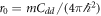${r}_{0}={{mC}}_{{dd}}/(4\pi {{\hslash }}^{2})$ and the scattering length a of the underlying effective two-body contact interaction. The constant C_dd measures the strength of the dipolar interaction; it is proportional to the square of the magnetic or electric dipolar moment. The ratio between r₀ and a shows that dipolar effects are weaker in magnetic systems than in heteronuclear polar molecules [9–11]. Production of these molecules is hindered by strong three-body losses but recent progress has been achieved with NaK [12] and NaRb [13]. Also very promising is the recent production of atomic BEC states of Dy [14–16] and Er [17, 18] that, with large magnetic moments, show stronger dipolar effects than the ones observed in Cr.

In three-dimensions (3D), the anisotropy of the interaction, with attractive regions, leads the system to an instability by collapse unless an additional repulsive hard core (or contact pseudopotential) is present. A delicate balance between these two terms can lead to the formation of self-bound droplets organized in a crystal lattice resembling the Rosensweig instability of classical ferrofluids [19–21]. In two-dimensions (2D), the collapse is avoided if the tilting angle formed by the polarization field and the direction normal to the plane of confinement is lower than a critical value ${\theta }_{c}$ . In this case, the interaction is fully repulsive but with a strength which depends on the direction of the distance vector. A similar effect is achieved in quasi-2D geometries when the perpendicular direction is tightly bound. Within the stability domain, one can observe new interesting features like the emergence of an exotic stripe phase [6].

In a more general sense, the anisotropy of the interaction is expected to affect most, if not all, the static and dynamic properties of the system. This includes the geometry of the crystal formed when brought to the solid phase, as in the classical case [22], and equivalently the spatial arrangement of a few-body dipolar system in the presence of a confining trap. A previous study based on exact diagonalization [22] has shown that already a three-particle system of (bosonic or fermionic) confined dipoles in quasi-2D geometries arrange in different spatial configurations as a function of the tilting angle. For the bosonic case, the three-particle system was also studied using the path integral ground-state Monte Carlo method [23]. Both studies, which arrived to the same solid-like configurations for bosons, were constrained to isotropic traps.

In the present work, we study the effects of the anisotropy of the dipolar interaction in a harmonically confined 2D few-body boson system. At difference with previous works [22, 23], we include two (sometimes competing) sources of anisotropy: one coming from the dipole–dipole interaction through the modulation of the polarization angle, and the other by using different frequencies in each axis of the confining trap. Therefore, we can generate situations where both anisotropies force particles to behave in the same way or, more interestingly, other ones where these two effects compete and favor different kind of arrangements. The results presented in this work correspond to the last case, where the competition between anisotropies produces a richer particle configuration scenario.

Our main goal is to identify the stable ground-state arrangements as a function of the tilting angle and trap anisotropy. Our study relies on the use of the diffusion Monte Carlo (DMC) method, which for bosons is exact within some statistical noise. From the experimental side, there are no available data on the few-body stable configurations of confined dipolar bosons. However, interesting and promising results involving the confinement of a few Rydberg atoms have been recently reported [24]. This experiment shows the formation of different patterns of confined atoms with an interaction potential proportional to $1/{r}^{6}$ instead of the $1/{r}^{3}$ dipolar one. On the other hand, anisotropic traps are routinely used in many experimental setups and thus the possible observation of the structures that we predict seems plausible.

The rest of the article is organized as follows. In the next section, we introduce the theoretical model under study and briefly describe the DMC method. In section 3, the main results are reported, paying special attention to the different regimes observed and to the comparison between the quantum and classical structures found in the simulations. Finally, section 4 comprises the main conclusions of our work.

2. Quantum Monte Carlo method

We simulate a few-body system of N harmonically confined bosonic dipoles of mass m under the action of the 2D Hamiltonian [11].

$\begin{eqnarray}\hat{H} & = & -\displaystyle \frac{{{\hslash }}^{2}}{2m}\displaystyle \sum _{i=1}^{N}{{\bf{\nabla }}}_{i}^{2}+\displaystyle \frac{m}{2}\displaystyle \sum _{j=1}^{N}({\omega }_{x}^{2}{x}_{j}^{2}+{\omega }_{y}^{2}{y}_{j}^{2})\\ & & +\displaystyle \frac{{C}_{{dd}}}{4\pi }\displaystyle \sum _{i\lt j}^{N}\displaystyle \frac{1-3{\sin }^{2}\alpha \,{\cos }^{2}{\theta }_{{ij}}}{{r}_{{ij}}^{3}},\end{eqnarray} \tag{ 2 }$

with $\{{r}_{{ij}},{\theta }_{{ij}}\}$ the interparticle distance and angle, corresponding to in-plane particle coordinates ${\vec{r}}_{j}=({x}_{j},{y}_{j})$ , $({\omega }_{x},{\omega }_{y})$ the trapping frequencies along the x and y axis, respectively, and α the tilting angle of the dipoles with respect to the axis perpendicular to the plane (in our case, the z axis). The polarization angle α is fixed and equal for all dipoles because the system is assumed to be fully polarized. Experimentally, this is achieved by applying an external electric or a magnetic field along the desired direction. We analyze the 2D system that could be realized as the limit of a quasi-2D geometry with an additional frequency ${\omega }_{z}\to \infty$ . The anisotropy of the dipole–dipole interaction shows up explicitly in the numerator of the last term (2), which becomes fully repulsive (with different strength in each direction) for all angles α fulfilling $1-3{\sin }^{2}\alpha \geqslant 0$ . Above a critical value ${\alpha }_{c}\sim 0.615$ the system collapses. Finally, it is also important to notice that by tunning ${\omega }_{x}$ and ${\omega }_{y}$ one introduces an additional source of anisotropy that can reinforce or compete with the anisotropy of the dipole–dipole interaction.

In order to reduce the variance in DMC simulations to a manageable level, the random walk in imaginary time is guided by a trial wave function that is used for importance sampling. In our work, we use a Bijl–Jastrow model,

$\begin{eqnarray}&&{{\rm{\Psi }}}_{T}({{\bf{r}}}_{1},\,\ldots ,\,{{\bf{r}}}_{N})=\displaystyle \prod _{i=1}^{N}{f}_{1}({{\bf{r}}}_{i})\displaystyle \prod _{j\lt k}^{N}{f}_{2}({{\bf{r}}}_{{jk}}).\end{eqnarray} \tag{ 3 }$

The one-body factor ${f}_{1}({\bf{r}})$ is taken as the exact wave function for a particle in the harmonic trap,

$\begin{eqnarray}&&{f}_{1}({\bf{r}})=\exp \left(-\displaystyle \frac{m}{2{\hslash }}({\omega }_{x}{x}^{2}+{\omega }_{y}{y}^{2})\right).\end{eqnarray} \tag{ 4 }$

The two-body correlation factor ${f}_{2}({{\bf{r}}}_{{jk}})$ is obtained from the solution of the zero-energy two-body Schrödinger equation without confinement [26],

$\begin{eqnarray}&&{f}_{2}({{\bf{r}}}_{{jk}})={f}_{0}({r}_{{jk}})+\displaystyle \sum _{n=1}^{\infty }2{f}_{2n}({r}_{{jk}})\cos (2n{\phi }_{{jk}}),\end{eqnarray} \tag{ 5 }$

with ${f}_{2n}({r}_{{jk}})$ the different partial-wave contribution corresponding to fixed angular momentum in 2D. We keep only the first terms of the expansion (5) as we have found that the inclusion of higher-order contributions do not change the results.

Hereafter, we use reduced units. Lengths are measured in harmonic oscillator units, with the characteristic length given by ${a}_{0}\equiv \sqrt{{\hslash }/(M\omega )}$ , and the characteristic energy given by ${E}_{0}={\hslash }\omega$ , M being the total mass of the system and $\omega \equiv \sqrt{{\omega }_{x}^{2}+{\omega }_{y}^{2}}$ . The strength of the dipolar interaction is written in terms of a dimensionless parameter λ,

$\begin{eqnarray}&&\lambda \equiv \displaystyle \frac{{C}_{{dd}}}{4\pi {\hslash }\omega {a}_{0}^{3}}.\end{eqnarray} \tag{ 6 }$

On the other hand, to account for the anisotropy of the confining trap we define the angle ${\theta }_{\omega }$ as

$\begin{eqnarray}&&\tan {\theta }_{\omega }\equiv \displaystyle \frac{{\omega }_{y}}{{\omega }_{x}}.\end{eqnarray} \tag{ 7 }$

These parameters, λ and ${\theta }_{\omega }$ , together with α, are the three most relevant quantities to characterize the structural behavior of the system.

3. Results

Our main goal is the determination of the most probable structures that appear when the system is strongly confined. We focus on the N = 3 and N = 4 cases and compare the quantum results obtained with the DMC method with classical ones derived from simulated annealing (SA) optimizations. In the latter case, we optimize the total (kinetic plus potential) energy on a given set of descending temperatures, to find the most stable configurations at $T\approx 0$ . This is equivalent to the minimization of the potential energy.

3.1. Quantum configurations

Our quantum simulations are based on a DMC program with a second-order propagator [25]. We have used a dimensionless time step ${\rm{\Delta }}\tau =0.01$ , measured in units of ${t}_{0}={E}_{0}/{\hslash }$ . Everywhere since we have verified that this single calculation is compatible with the quadratic extrapolation to ${\rm{\Delta }}t\to 0$ . We work with an average number of walkers N_w = 1200 and N_w = 400 for N = 3 and N = 4, respectively. Larger populations produce results that are indistinguishable within the characteristic statistical noise. From preliminary simulations, we determined the minimum strength required to stabilize solid-like patterns, which correspond to $\lambda =1039$ and $\lambda =1600$ for N = 3 and N = 4, respectively. In the following, we set λ to these values.

To elaborate on the different observed patterns, we have to properly identify the regions of the parametric space (α, ${\theta }_{\omega }$ ) where each structure is stable. We consider a particular structure to be stable when their geometric properties do not change significantly under slight variations of α and ${\theta }_{\omega }$ . To determine these regions, and the corresponding transitions between them, we rely on two criteria: geometry and energy. The first criterion consists on looking at each particle density distribution and to classify it according to the shape of the formed arrangement. In order be more precise than just looking at the patterns found, we estimate the cosines of the angles formed by the relative position vectors between different particles, 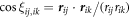$\cos {\xi }_{{ij},{ik}}={{\bf{r}}}_{{ij}}\cdot {{\bf{r}}}_{{ik}}/({r}_{{ij}}{r}_{{ik}})$ . All configurations in the parametric space $(\alpha ,\ {\theta }_{\omega })$ are considered to be of the same type when the condition

$\begin{eqnarray}&&| {(\cos {\xi }_{{ij},{ik}})}_{{\alpha }^{(1)},{\theta }_{\omega }^{(1)}}-{(\cos {\xi }_{{ij},{ik}})}_{{\alpha }^{(2)},{\theta }_{\omega }^{(2)}}| \lt \delta ,\forall \ i,j,k\end{eqnarray} \tag{ 8 }$

is satisfied for a suitable value δ. In this condition, δ is a selection parameter, typicality small. In our case, it has been set to $\delta =0.07$ , as we have found this value to accurately separate the different solid-like patterns, in agreement with the energetic criterion discussed below.

As an example, we report in table 1 the values of these cosines for different points in the (α, ${\theta }_{\omega }$ ) plane for fixed λ and N = 4 in regimes A, B, and D (see figure 5). In figure 1, we show an example of this structure, with labels on the particle positions, to illustrate which angles are measured. We can see that the difference of the values of the cosines between different patterns is clear allowing for their classification.

**Figure 1.** Structures corresponding to the particle configurations of table 1. Numbers label particles while letters indicate the corresponding region. Since the structures in region D are degenerated, we show one of the possible configurations. The horizontal and vertical axes corresponds to the x and y coordinates respectively, and are expressed in reduced units.
Download figure:
Standard image High-resolution image

Table 1. Cosines of different angles formed by relative particle position vectors for different points of the parametric space (α, ${\theta }_{\omega }$ ) belonging to patterns A, B and D, with N = 4.

Region	A		B	D
Point	$\alpha =0.2$ , ${\theta }_{\omega }=26.25^\circ$	$\alpha =0.5$ , ${\theta }_{\omega }=20^\circ$	$\alpha =0.2$ , ${\theta }_{\omega }=20^\circ$	$\alpha =0.2$ , ${\theta }_{\omega }=45^\circ$
$\cos {\xi }_{\mathrm{21,24}}$	−0.6383 ± 0.0021	−0.6701 ± 0.0013	0.9050 ± 0.0033	−0.0178 ± 0.001
$\cos {\xi }_{\mathrm{12,13}}$	0.6647 ± 0.0011	0.7067 ± 0.0008	−0.9167 ± 0.0015	0.0341 ± 0.0012
$\cos {\xi }_{\mathrm{42,43}}$	0.6592 ± 0.0027	0.6732 ± 0.0022	−0.9507 ± 0.0010	0.0263 ± 0.0008

Relevant information about structural changes is also reflected in the behavior of the energy. We have calculated the energy of the different patterns for a wide range of (α, ${\theta }_{\omega }$ ) values, and the results obtained are shown in figure 2. The point where the energy shows a kink determines the stability boundary of a given structure in the (α, ${\theta }_{\omega }$ ) plane for a fixed λ value. When a change in the spatial configuration is produced, the derivative of the energy changes discontinuously, generating the kink. However, sometimes the change in the slope is so small that it can hardly be seen in figure 2. This is the case, for example, with the transition at $\alpha =0.6$ , ${\theta }_{\omega }\simeq 30^\circ$ shown in the upper panel in figure 6.

**Figure 2.** Ground-state energy as a function of the anisotropy of the confining trap ( ${\theta }_{\omega }$ ) for different values of the tilting angle α. Top and bottom panels correspond to the N = 3 and N = 4 systems, respectively.
Download figure:
Standard image High-resolution image

**Figure 2.** Ground-state energy as a function of the anisotropy of the confining trap ( ${\theta }_{\omega }$ ) for different values of the tilting angle α. Top and bottom panels correspond to the N = 3 and N = 4 systems, respectively.
Download figure:
Standard image High-resolution image

The stable structures for N = 3 are shown in figure 3. We observe four different patterns that we label as A, B, C, and D. Each one of the first three structures is stable in shape within a certain domain of the parameter space here explored. However, the last one D is not as stable as the other three. In figure 3, we show two D patterns emerging from two different (α, ${\theta }_{\omega }$ ) points. The shape of both configurations is slightly different: the one of the left corresponds to a rotating equilateral triangle producing a circular ring while the right one shows an elliptical shape. The rotating equilateral triangle does only arise when the trap is spherically symmetric (i.e. ${\theta }_{\omega }=45^\circ$ ), while the elliptical shape appears in the rest of the D region. Despite this difference, we decided to consider both diagrams of the same family type since both correspond to highly degenerate triangle structures. Our decision is complemented by the results that we have obtained for the two-body distribution function g(r), which is proportional to the probability of finding two particles at a distance r averaged over all angles. Explicitly,

$\begin{eqnarray}&&g(r)={{ \mathcal N }}^{-1}\,\langle \displaystyle \sum _{i\ne j}^{N}\delta (r-{r}_{{ij}})\rangle ,\end{eqnarray} \tag{ 9 }$

with ${ \mathcal N }$ a normalization constant. In figure 4, we report g(r) for the circular and elliptical shapes of D type and for a typical C structure. As we can see, D structures show only one broad peak resulting from the average of the different triangular configurations, whereas C has two due to its aligned pattern. It is worth noticing that for ${\theta }_{\omega }=45^\circ$ (isotropic trap) we reproduce the structures reported previously in [22, 23] with a slight shift in the transitions due to our more tight confinement.

**Figure 3.** Quantum particle density distributions for N = 3. Labels denote the corresponding region in the quantum structural diagram of figure 6. In the second row, we plot two D configurations to illustrate the changes that the structure experiment over its stability domain. The horizontal and vertical axes corresponds to the x and y coordinates respectively, and are expressed in reduced units.
Download figure:
Standard image High-resolution image

Increasing the number of particles from 3 to 4 produces more stable structures. This is shown in figure 5, where we report illustrative examples of the stable patterns found, labeled A to F. Notice that the D structure corresponds to a square configuration under rotation, similar in shape to the degenerate equilateral triangle observed in the D structure for N = 3.

In figures 6 and 7 we draw the N = 3 and N = 4 stability domains of the different structures in the ( ${\theta }_{\omega }$ , α) plane. The boundaries of different regions are approximate because transitions between particle arrangements are not characterized by abrupt discontinuities of any order parameter. We draw a line to guide the eye and help to distinguish neighboring structures; this line is thicker in the boundaries of the quantum structures than in the classical ones because quantum transitions are in general more progressive. Anyway, our results point to a rich scenario, specially in the region of large tilting angle α. For instance, when $\alpha \simeq 0.6$ we count up to five different patterns for N = 4 and four for N = 3 by changing the geometry of the confining trap. This is reduced to three and two for N = 4 and 3, respectively, in the isotropic case $\alpha =0$ .

**Figure 6.** Structural diagrams for the quantum (top) and classical (bottom) cases for N = 3. The vertical axis corresponds to ${\theta }_{\omega }$ , expressed in degrees, while the horizontal axis corresponds to α, expressed in radians. The dashed lines are a guide to the eye to better distinguish neighboring structures.
Download figure:
Standard image High-resolution image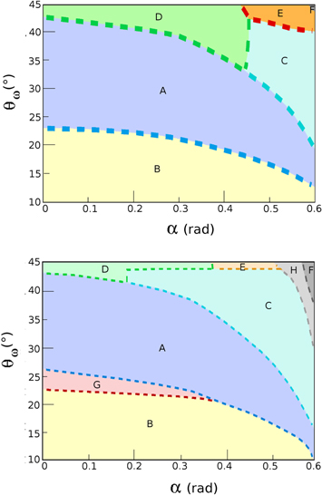

**Figure 7.** Same as in figure 6, for N = 4 particles.
Download figure:
Standard image High-resolution image

The value of the trap strength ω corresponding to the diagrams presented in figures 6 and 7 depends on the dipole moment of the particles. The actual values required to observe some of the effects reported here are unfortunately out of reach with actual magnetic atoms. However, it may be possible to realize them with polar molecules (which have orders of magnitude larger dipolar moments) once the difficulties associated to chemical reactions and three-body losses are sorted out [27, 28]. Despite these experimental issues, we provide the value of the necessary trap strength for two different species of polar molecules used in experiments: ⁸⁷Rb¹³³Cs [29], which possesses an intrinsic dipole moment of 1.25 D, requires a trap strength of $\omega =71.245\,\mathrm{kHz}$ and ²³Na⁸⁷Rb [13], with an intrinsic dipole moment of 3.2 D, requires of $\omega =13.539\,\mathrm{kHz}$ . These values are calculated assuming that the induced electric dipole moments of the molecules are equal to the intrinsic ones, while the ones that can be achieved in present experiments are somewhat lower. According to other theoretical works [22], it is even possible to use less tight traps at the expense of finding more diffuse results.

3.2. Quantum versus classical patterns

It is interesting to determine the relevance of quantum effects on the different structures that we have found using the DMC method. To this end, we have performed classical calculations to find the optimal patterns for different values of parameters ${\theta }_{\omega }$ and α. This analysis has been carried out using the SA optimization method. Figures 8 and 9 show the complete set of structures found for N = 3 and N = 4, respectively. The slight dispersion around the optimal coordinates is a direct measure of the space binning employed.

**Figure 8.** Classical patterns for N = 3. Labels tag the corresponding regions in the structural diagram of figure 6. The horizontal and vertical axes show the x and y coordinates, respectively.
Download figure:
Standard image High-resolution image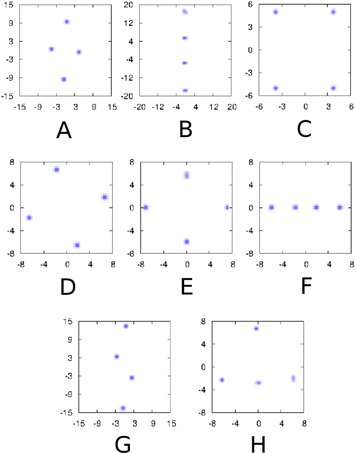

**Figure 9.** Classical patterns for N = 4. The labels correspond to their corresponding region in the classical structural diagram shown in figure 7. The horizontal and vertical axes corresponds to the x and y coordinates respectively, and are expressed in reduced units.
Download figure:
Standard image High-resolution image

From the comparison between the quantum and classical structures one can establish the main differences between them. We see that, for the same number of particles, there are more classical structures than quantum ones, while the classical and quantum transition regions between different structures do not coincide. Furthermore, structural transitions are more progressive in the quantum case than in the classical one, meaning by progressive that in the quantum simulation there is a larger parametric region featuring non stable structures between two stable ones.

The key factor explaining these differences is the quantum kinetic energy, which is absent in the classical system at zero temperature. This effect explains why the number of structures is greater in the classical case than in the quantum one, since the kinetic energy contributes to particle diffusion rather than localization, making some structures be less stable. As an example, the classical patterns G and H for N = 4 are absent in the quantum case. In a similar way, the classical structure E does not appear in the quantum diagram for N = 3. Quantum motion is also responsible for the more progressive behavior of quantum transitions as it favors delocalization. It is important to remark that the classical structures of region D for both N = 3 and N = 4 are degenerated, just like its quantum counterparts. However, in the figures we just plot one of the degenerated structures.

Regarding the evolution with the number of particles, we observe that the quantum and classical patterns are more similar in the four particle case than in the three particle one. For fixed trap parameters, interparticle distances are smaller for N = 4 than for N = 3, thus increasing the potential energy contribution (localization) with respect to the kinetic one (dispersion).

3.3. Change of interaction strength

Up to this point, we have kept fixed the interaction strength λ. In this subsection, we analyze the influence of λ on the results. In fact, the change of λ, for fixed trapping frequencies, mainly modifies the ratio between the potential and kinetic energies. A stronger dipolar strength for a given trap implies that the contribution of the potential energy increases over the kinetic one. In some sense, that means that the system approaches a more classical scenario, where all the energy at T = 0 is potential. On the contrary, by decreasing λ the potential contribution is reduced and the system is more delocalized. This feature can be observed by looking at the DMC particle densities for fixed (α, ${\theta }_{\omega }$ ) as a function of λ. We report in figure 10 the density profiles for $\alpha =0.6$ , ${\theta }_{\omega }=45^\circ$ and N = 4. For the sake of comparison, the corresponding classical pattern is also shown. The evolution with λ shows less localized patterns the lower the trapping strength; a somewhat ordered configuration at $\lambda =237$ and a particle arrangement very similar to the classical one at $\lambda =1600$ . Therefore, we observe a transition from a quantum gas to a quasi-solid structure, which resembles the classical solution.

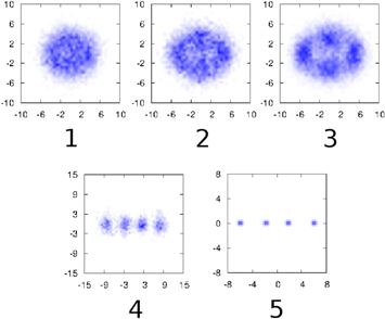
**Figure 10.** Density profiles for $\alpha =0.6$ and ${\theta }_{\omega }=45^\circ$ for different λ values. The structures from left to right and from top to bottom correspond to $\lambda =40$ , $\lambda =120$ , $\lambda =237$ and $\lambda =1600$ . Bottom right structure is a SA histogram showing the classical minimum energy structure for $\lambda =1600$ . The horizontal and vertical axes corresponds to the x and y coordinates respectively, and are expressed in reduced units of position.
Download figure:
Standard image High-resolution image

**Figure 10.** Density profiles for $\alpha =0.6$ and ${\theta }_{\omega }=45^\circ$ for different λ values. The structures from left to right and from top to bottom correspond to $\lambda =40$ , $\lambda =120$ , $\lambda =237$ and $\lambda =1600$ . Bottom right structure is a SA histogram showing the classical minimum energy structure for $\lambda =1600$ . The horizontal and vertical axes corresponds to the x and y coordinates respectively, and are expressed in reduced units of position.
Download figure:
Standard image High-resolution image

Finally, and in order to show this evolution in a more quantitative way, we report in figure 11 a plot of the ratio of the kinetic to the potential energies ${E}_{{\rm{k}}}/{E}_{{\rm{p}}}$ , for N = 4, in terms of $\lambda /N$ for two sets of $(\alpha ,\ {\theta }_{\omega })$ values: ${P}_{1}=\{\alpha =0.6$ , ${\theta }_{\omega }=45^\circ \}$ (same as in figure 10) and ${P}_{2}=\{\alpha =0.5$ , ${\theta }_{\omega }=30^\circ \}$ . We have chosen these two points only because they present two different and generic situations. In P₁, increasing the strength of the interaction makes the system undergo a structural change, visible in a change of the tendency of the ratio of energies around $\lambda /N\sim 300$ . This is not the case for point P₂, where the system always remains in the same structural configuration. The change of energy ratios in point P₁ is due to the fact that, when the transition is produced, the competing structures have the same total energy. However, due to their geometry, they have different potential contribution, which in turn induces a corresponding change in the kinetic energy. In this way, both quantities change abruptly and this leads to the noticeable bump in the curve. Looking at figure 10, we can see that the change from a structure of the type 3 to a structure of the type 4 is the cause of the aforementioned discontinuity. Once again, this situation is representative of what happens in other points of the diagram. It is also interesting to compare the quantum and classical energies at the same points (α, ${\theta }_{\omega }$ ) of the parametric space. This is shown in figure 12 for the same conditions than in figure 11. As one can see, the ratio of quantum to classical energies, ${E}_{{\rm{q}}}/{E}_{{\rm{c}}}$ , is larger than one but slowly tends to unity when approaching the classical limit. This happens when the trapping strength increases for fixed $(\alpha ,{\theta }_{\omega })$ . The ratio tends to one but, in the regime of interaction parameters studied here, it is still significantly larger, mainly in aligned configurations.

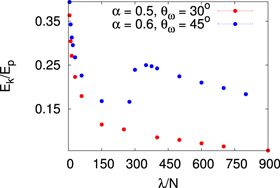
**Figure 11.** ${E}_{{\rm{k}}}/{E}_{{\rm{p}}}$ as a function of $\tfrac{\lambda }{N}$ for two points of the parametric space (α, ${\theta }_{\omega }$ ).
Download figure:
Standard image High-resolution image

**Figure 12.** Ratio ${E}_{{\rm{q}}}/{E}_{{\rm{c}}}$ of quantum (E_q) to classical $({E}_{{\rm{c}}})$ energies as a function of $\lambda /N$ for two points of the parametric space (α, ${\theta }_{\omega }$ ).
Download figure:
Standard image High-resolution image

**Figure 12.** Ratio ${E}_{{\rm{q}}}/{E}_{{\rm{c}}}$ of quantum (E_q) to classical $({E}_{{\rm{c}}})$ energies as a function of $\lambda /N$ for two points of the parametric space (α, ${\theta }_{\omega }$ ).
Download figure:
Standard image High-resolution image

4. Conclusions

Using the DMC method, that allows for an exact description of Bose quantum systems, we have studied the different structures that appear when a few-body system of dipoles (N = 3 and N = 4) is harmonically confined. The analysis has been carried out by changing the two sources of anisotropy of the problem: the confining harmonic potential and the dipolar interaction strength. The combination of these two effects produce a collection of different patterns whose stability domains and boundaries have been established.

In order to know if the different quantum structures have a corresponding classical counterpart, we have carried out extensive optimization searches using the SA method. Our results show that the main differences between the quantum and classical structures are: (a) a greater number of particle arrangements appear in the classical case, (b) a noticeable difference in the location of boundaries between similar structures in the classical and quantum cases, and (c) a more progressive character of the quantum transitions between structures. The quantum kinetic energy seems to be the determining factor for understanding all these differences.

We have also shown that the interaction strength influences on the ratio between the kinetic and potential energies. When the strength λ grows, the potential energy becomes more relevant, leading the system to a more classical scenario. On the contrary, by decreasing λ the quantum system delocalizes due to the dominant role of the kinetic energy, and thus it departs completely from the classical zero-temperature solid-like configuration.

Acknowledgments

This research was supported by MINECO (Spain) Grant No. FIS2014-56257-C2-1-P.

Few trapped quantum dipoles: quantum versus classical structures

Article metrics

Author e-mails

Author affiliations

Author notes

Dates

Abstract

1. Introduction

2. Quantum Monte Carlo method