


Abstract
We present a completely analytical vortex-fluid model describing several vortex-fluid phases of hole-doped cuprate superconductors below and above Tc. A key feature of the model is to synthesize several vortex damping mechanisms of scattering inside vortex core, core–core collisions and pinning. Accurate predictions for both magnetoresistance and Nernst effect are obtained, validated by measurements in six Bi-based cuprate samples over a wide range of temperature and magnetic fields, which strongly support the phase-fluctuation scenario in Bi-based cuprates. The model quantifies the unconventional vortex properties by a set of physical parameters, which adds quantitative contents to the discussions of pseudogap. A speculation is offered to use the vortex-fluid model as a first step towards achieving a comprehensive understanding of Nernst effect for all HTSC.
Export citation and abstract BibTeX RIS

Original content from this work may be used under the terms of the Creative Commons Attribution 3.0 licence. Any further distribution of this work must maintain attribution to the author(s) and the title of the work, journal citation and DOI.
1. Introduction
It is well known that transport properties are powerful tools to address the pseudogap problem in high-temperature superconductors (HTSC) [1, 2]. A remarkable property is the so-called Nernst effect [3], in which a conductor exhibits a transverse detectable voltage when magnetic field is applied along  direction perpendicular to the direction of temperature gradient. In a conventional superconductor, large Nernst signal below Tc is a sign of vortex transport. But it was somewhat unexpected that strong Nernst signal were experimentally discovered above Tc in HTSC [4, 5], which has since stimulated extensive discussions on the nature of pseudogap state, e.g. superconducting fluctuations or competing order. Generally speaking, there are mainly three possible candidates, i.e., vortices [6, 7], fluctuating Cooper pairs [8], and quasiparticles (qp) generated from depair effect. A central issue in the study of hole-doped HTSC is thus: which component dominates the origin of Nernst signal in pseudogap state?
In underdoped cuprate, one typically observes positive qp Nernst signal above Tc and usual negative qp signal at very high temperature. A linear field dependence of positive Nernst signals is observed in a wide field regime at well above Tc in underdoped  SrxCuO4 (LSCO) and Eu-LSCO [5, 9], which is interpreted as a proof to support the qp scenario, which is thought [10–12] to originate from density wave order [13–15]. The theoretical prediction of peak signal variation with temperature reproduces qualitatively the observed behavior in experiments. However, the qp signal is not accurately quantified near or below Tc, due to the fact that remarkable contributions of superconducting fluctuations to conductivity are neglected. Thus, the parametrization and validation of qp models call for a quantification of the superconducting fluctuations.
Gaussian fluctuations are conventional scenario due to fluctuating Cooper pairs above Tc, which is analyzed by Ussishkin et al [8] in low fields of LSCO, and later, extended by a microscopic theory to describe temperature and field dependence for arbitrary temperatures and magnetic fields of NbSi, Eu-LSCO and PCCO [9, 16–18]. At low fields near Tc, the signal of fluctuating Cooper pairs expressed by  (thermoelectric coefficient over field) is proportional to the square of coherence length, which is large in NbSi (conventional superconductors) and PCCO (electron-doped cuprate), and thus superconducting fluctuations are dominated by Gaussian fluctuations in these samples. On the other hand,
  must be smaller in most hole-doped cuprates due to their smaller coherence lengths. Indeed, experimentally observed signals are small in overdoped LSCO, as correctly predicted by the Gaussian-fluctuation theory. However, in underdoped LSCO and nearly optimally doped Bi-2212, Gaussian-fluctuation theory generally underestimates the signal (see section 3.1.3), which indicates an evidence that phase fluctuations are more important in these samples. We will show that the contribution of Gaussian fluctuations is minor in pseudogap state of hole-doped cuprates.
Due to two dimensionality (2D), low carrier density and short coherence length, phase fluctuations are believed to be especially strong in underdoped cuprates. According to the phase-fluctuation scenario [19], superconductivity is terminated at Tc due to proliferation of thermal vortices. Nevertheless, local phase coherence is still present, driving a substantial vortex Nernst signal until upper critical temperature Tv and field  [5, 6, 20] are reached. Experimentally, the widely observed tilted-hill profile of Nernst data and the continuity below and above Tc are strong evidences for the existence of vortices. Theoretically, 2D XY model [7] and time-dependent Ginzburg–Landau (TDGL) equation [21–24] have been studied for transverse thermoelectric coefficient, but successful comparison is quantitatively achieved only in limited regimes, i.e., at at low field and high temperature in underdoped LSCO and at high fields and low temperature in overdoped LSCO. Furthermore, thermoelectric coefficient does not specify the whole transport; without the description of vortex damping, direct prediction of Nernst signal is not possible in these simulation studies.
In order to develop a whole description of the Nernst signal, Anderson proposed a phenomenological theory of vortex-tangles in pseudogap state [25]. However, an estimate indicates that his model presents an overestimation of two orders of magnitude in predicted resistivity compared to magnetoresistance data [26]. Thus, the validity of the vortex concept or phase-fluctuation scenario in pseudogap state remains to be established in a quantitative manner. In summary, it seems that there exists no quantitative theory capable of describing the Nernst signal for pseudogap state over the wide range of temperature and magnetic field. In our view, the situation originates from an oversimplification of the subject, i.e., insisting on finding a simple and single origin for describing the various samples and phase regimes. In fact, HTSC is a system composed of complicated physical environment where there are interplays between several interacting components, including several driven and damping mechanisms due to impurity and external fields. What is needed is a comprehensive theory synthesizing the three currents, in the light of quantitative measurements in a wide range of T, B and with doping dependence. The theory should assert quantitatively at the end what are dominant components in different regimes, and what are the transitions between the multiple regimes in the B–T phase diagram.
It is widely recognized that vortex fluid is the dominant component below Tc, thus a quantitatively accurate vortex-fluid model is the first step before achieving the comprehensive theory. In other words, without a proper quantification of vortex signal, the parametrization of HTSC physics is not reliable. We hereby attempt to build a sound vortex-fluid model which will serve as a basis for building a more complete theory, taking into account contributions of qp and amplitude fluctuations. In the present work, we focus on Bi-based cuprates in which vortex Nernst signal is the dominant contribution in most regimes, thus the vortex-fluid model can be quantitatively verified. Note that Bi-cuprates are extremely 2D superconductors in which phase fluctuations are strong, the qp signals are experimentally found to be small [5], and the Gaussian fluctuations are suppressed due to small coherence length. Experimentally, the onset temperature of pseudogap  is much higher than Tc in most doping of Bi-based cuprates [27, 28], indicating that amplitude fluctuations do not significantly affect the physics around Tc. Therefore, we expect that the vortex model alone can explain the Nernst signal over most regimes discussed below.
The main task in constructing a quantitative description of vortex Nernst signal is to model the complex damping process associated with vortex motions, which needs to go beyond Bardeen–Stephen model. Based on our recent work [26] which proposes a core–core collisions mechanism of vortex tangles, an unified vortex damping formula modeling several processes including scattering inside vortex core, core–core collisions and pinning is achieved, enabling accurate predictions of both magnetoresistance and Nernst signal over a wide range of T and B. During the process of fitting a wide range of data, we have developed a systematic procedure, to determine several physical parameters which quantify the unconventional vortex properties in pseudogap state. The success yields a solid support to the underlying picture of vortex fluid in pseudogap state proposed by Anderson [6, 25, 29], as well as builds a basis for the comprehensive theory of transport integrating all three components in HTSC.
The paper is organized as follows. In section 2, an unified model is defined to quantify the damping viscosity, and to describe flux-flow resistivity and Nernst effect. In section 3, the model is first verified against magnetoresistance and Nernst data; for comparison, the validity of the Gaussian model is also assessed. Then, several physical parameters are discussed, displaying in particular the unconventional vortex properties in pseudogap state. Section 4 is devoted to the discussions on further applications and on the mechanism study of entropy.
In this work, HTSC refers to cuprate superconductors mostly and iron-based superconductors only in section 4. Some other acronyms are used to identify the cuprates, Bi-2201 for Bi2 LayCuO6, Bi-2212 for Bi2Sr2CaCu2O
 , UD, OP, and OV stand for underdoped, optimally doped, and overdoped, respectively.
2. Model description
2.1. Flux-flow resistivity
Consider a quasi-2D cuprate superconductor, and choose Tc as the Berezinskii-Kosterlitz-Thouless (BKT) phase transition temperature [30–32]. When magnetic field is applied in HTSC, there are two types of vortices, namely magnetic and thermal vortices, whose density will be denoted as  and nT. Since the thermal vortices appear in pairs, the density of vortices is
  , and that of antivortices (with a reversed angular momentum) is
  .
.
In the experiment of flux-flow resistivity as schematically described in figure 1, a transport current density j is applied  and magnetic field H
 . A vortex current perpendicular to j is driven by a Lorentz force fL = j
  , where c is the speed of light. And in the steady state, fL must be balanced by a damping force, e.g., for a vortex,

where η is the damping viscosity per unit length and vϕ is the drifting velocity of the vortex. Vortex flow generates a phase slippage [33, 34], which induces transverse electric fields  , where
  is the total vortex density. Here, both vortex and antivortex contribute to the total electric field since they transport in opposite directions. Thus, the flux-flow resistivity ρ can be derived as [35]

In equation (2), two key parameters are involved, namely the damping viscosity η and the thermal vortex density nT.

Figure 1. Schematic picture of the electric field E induced by the vortex flow under a driven current j. There are two types of vortices and velocity  , where + and − represent vortex and antivortex respectively.
Download figure:
Standard image High-resolution imageAbove Tc, nT can be determined by vortex correlation length  as
as  , where
  represents the characteristic scale beyond which thermal vortices begin to unbind [36]. At
  , superconducting fluctuations dominate, thus we speculate that the superconducting fluctuations make thermal vortices undergo a critical behavior. This behavior is studied by Kosterlitz [37], and follow his idea, we can define the following effective fields for modeling effects of thermal vortices:

where Bl represents the high-temperature limit of BT. In a special situation when  , BT saturates quickly to Bl at
  . Thus, at the high-temperature limit, the thermal vortices is as dense as the critical state described by
  , where
  is the upper critical field at
  . Thus, we can assume
  and use this approximation to achieve the comparison between theoretical predictions and experimental data.
2.2. Vortex Nernst effect
In figure 2, a temperature gradient  is applied
  and magnetic field H
 . As vortex contains higher entropy (and heat) than surrounding fluid, thus a vortex flow is driven by
  . This results in a heat transport with an energy
  , where Sϕ is the transport entropy per unit length of a vortex [38, 39]. In the steady state, thermal force should be balanced by damping force,

Thermal diffusion and the transport velocity is the same for vortices and anti-vortices as they have the same thermodynamic properties, as illustrated in figure 2. Thus, their contributions of phase slippage cancel with each other. Then, only the magnetic vortices contributes to Nernst signal  , then


Figure 2. Schematic diagram of Nernst effect. Vortices and antivortices are driven by temperature gradient  to form a flux flow, and then results in a Josephson voltage perpendicular to
  .
.
Download figure:
Standard image High-resolution imageThe origin of Sϕ is still under debate in the literature [39]. Nevertheless, inspired by Anderson's simple idea based on BKT scenario near Tc, it is possible to develop an order-disorder balance argument to obtain an expression for Sϕ in a dense vortex fluid, as we do now. In the superconducting state, the ordered motions (e.g., the supercurrents) obviously dominate over disordered motions (e.g., the qp currents), while it is the opposite in the normal state. In a 2D dense vortex fluid in Bi-based cuprates, strong phase fluctuations induce frequent vortex creation and annihilation, which yields an energy transfer and then a balance between ordered motions (i.e. the kinetic energy of supercurrents, Ek) and disordered motions (i.e. the heat,  ) in a vortex. Thus,
  . Neglecting the Kosterlitz–Thouless screening [32], the kinetic energy can be obtained by an integration from vortex core size ξ to
  ,
,

where ns is the local superfluid density,  cm4 gs−2, c0 is the c-axis lattice constant [40], and the effective mass of the hole is assumed as electron mass me. Note that the above balance argument is an extension of the BKT scenario, but we neglect the ordered motions inside the vortex core owing to cheap vortices scenario [41].
2.3. Damping model
The key theoretical contribution of the present work is the unified vortex damping model proposed in this subsection. Generally speaking, damping viscosity η involves several mechanisms, which are difficult to calculate from the first principle, and will then be considered with phenomenological arguments. Three damping mechanisms are considered, namely impurity (or defect) scattering of qp inside the vortex core, core–core collisions, and an interaction between vortex and pinning center. We assume that these three mechanisms can be decomposed so that η can be expressed as their linear superpositions,

where  ,
,  and
and  are the contribution of impurity scattering, vortex–vortex collision and pinning, respectively.
2.3.1. Impurity scattering of qp
Since the number of qp inside vortex core (about 10 holes in OP Bi-2212) and the phonon density at low temperature are both small, the scattering between phonon and qp inside vortex core is negligible in a vortex fluid below Tc. In this case, damping inside vortex core is dominated by impurity scattering, which is approximately temperature-independent. Thus,  should be a constant for a given material, which can be expressed as
  where
where  is a characteristic resistivity. The steep rises above melting field in experiments [5] indicates that vortices move very fast in a dilute vortex fluid, thus
  should be much bigger than the normal state resistivity considered in Bardeen–Stephen model [42].
2.3.2. Core–core collisions
The crucial difference between HTSC and conventional SC is that for HTSC, core–core collisions are more important due to much higher vortex density under small coherence length. While the independent vortex assumption may be valid in low fields, it is certainly inappropriate in high fields in cuprates. When the sample is tested in high fields (say B = 10 T), the distance between vortex cores  becomes of the order of 100 Å, which is much smaller than the penetration depth
  . Thus, vortices strongly interact with each other, leading to a remarkable increase of damping. In our recent work [26], we propose a new mechanism of core–core collision in dense vortex fluids: two vortex cores merge together to a bigger core, leading to an increase of qp DOS. This process induces a momentum transfer from circular supercurrents to qp, and then a damping. Since the random motion of vortex core originates from quantum fluctuations of holes [26], the mean-free-path of the core–core collision is proportional to reciprocal of core density. Thus, a dimensional argument yields a linear nv dependence of
  ,
,

where  is a characteristic normal state resistivity. This new mechanism offers an explanation [26] of a longstanding puzzle, i.e. the unconventional vortex dissipation in cuprate superconductors, as well as the nature of the discrepancy of Anderson's damping model.
Express  also in terms of
  , we obtain

where  is the effective fields to describe the damping strength of impurity scattering relative to core–core collisions.
2.3.3. Pinning effect
Pinning effect introduces modification to the transport of a vortex fluid [43]. According to Blatter et al [43], pinning effect can be expressed in an effective damping viscosity. Since pinning and core–core collisions both depend on inter-vortex distance, their joint effect can then be written in terms of a multiplicative factor Γ such that  The value of Γ must satisfy two limiting conditions. First, at high temperature and strong fields limit where the pinning effect vanishes, Γ is equal to 1. At low temperature and weak field limit, it is the thermal assisted flux flow (TAFF) described by Arrhenius law
 ![$\rho \approx {\rho }_{0}\exp [-{U}_{{\rm{pl}}}/({k}_{B}T)]$](https://content.cld.iop.org/journals/1367-2630/19/11/113028/revision2/njpaa8ceeieqn55.gif) , where Upl is the plastic deformation energy [43, 44]. A simple choice is thus
, where Upl is the plastic deformation energy [43, 44]. A simple choice is thus  , which yields the following expression:

The B and T dependence of Upl may vary with samples [43, 45], which has been parameterized by Geshkenbein et al in terms of an energy involving deformations of the vortex lines on a scale of inter-vortices distance [46]. We introduce a parameter Bp as an effective field strength quantifying pinning. Then, the model of Geshkenbein et al can be expressed as

Note that this kind of B and T dependence was indeed discovered experimentally in Bi-2212 [47, 48]. Therefore, in the sequel, we use equation (11) to describe the pinning effect in Bi-based cuprates. Bp is an intrinsic material parameter, which can be probed by the melting field Hm as  according to Lindemann criterion [43, 49], where cL is the Lindemann number and
  .
.
Finally, the total damping can be written as

2.4. Final model

![${B}_{T}={B}_{l}\exp [-2b| T/{T}_{{\rm{c}}}-1{| }^{-1/2}]$](https://content.cld.iop.org/journals/1367-2630/19/11/113028/revision2/njpaa8ceeieqn59.gif)


3. Results
3.1. Validation and comparison
3.1.1. Magnetoresistance
In this section, in-plane magnetoresistance is used to validate our damping model. In OP ( ) sample of
  , ρ is measured in a wide range of temperature (20–120 K) and fields (0–17.5 T) [50]. As is shown in figure 3, ρ first shows a slow increase regime at low temperature, which is a TAFF regime, and then the curves converge at a characteristic temperature. The transition between the two regimes varies with H. Equation (13) is applied to describe the data, see solid lines in figure 3, showing very good agreement at all five magnetic field values. The agreement is specially good at H = 0, where all vortices are thermal. Thus, our model of ρ is clearly validated.

Figure 3. Comparison between predictions (solid line) and experimental data (symbols) [50] using the fine tuned parameters given in table 1 at H = 0, 0.5, 3, 9, 17.5 T. Only the data at  K are fitted.
Download figure:
Standard image High-resolution imageSince the formula involves seven parameters, a systematic procedure must be developed to determine them. A two-step procedure is developed, with a rough estimate (RE) first and then a fine tuning (see appendix A.1 for a detailed presentation). Note that this determination is not an arbitrary fitting, but involves a careful asymptotic analysis, which ensures the uniqueness of the outcome. The main idea can be summarized as follows. First, a RE is conducted using asymptotical analysis at large and small limits of T and B; at each limit, only one or two parameters appear, so that the parameter values can be easily determined. Applying all limiting data yields a complete set of RE values, which are then subjected to a fine tuning (FT) process, involving a search for optimal parameters around the RE values, minimizing the errors between the set of predictions and data. At the end of the FT step, precise parameter values are obtained, and its uncertainties are assessed, see table 1.
Table 1.
Material parameters in equation (13) determined in two steps, rough estimate (RE) and fine tuning (FT), described in appendix, for  . [50] The uncertainty is calculated by first setting all parameters to be their FT-determined values, and then varying only one given parameter to observe the root mean square fitting error equal to the experimental uncertainty, i.e.,
  cm.
cm.
| Step | Tc (K) |
 (mΩ cm) (mΩ cm) |
Tv (K) | B0 (T) | Bp (T) | Bl (T) | b | RMSE ( cm) cm) |
|---|---|---|---|---|---|---|---|---|
| RE | 87 | 0.116 | 112 | 4 | 30.8 | 68.1 | 0.42 | 10 |
| FT | 87 | 0.099 ± 0.11 | 104 ± 3 | 0.4 ± 0.4 | 89 ± 34 | 68.1 | 0.56 ± 0.11 | 5 |
Let us discuss the reliability of each parameter determination. First, the upper critical temperature Tv is the onset temperature of short-range coherence and thermal vortices, when decreasing the temperature. In the vortex-fluid model, it indicates the temperature, beyond which the vortex magnetoresistance collapses and vortex Nernst signal vanishes. Using the data of Usui et al, Tv = 112 K is obtained in RE and corrected to 104 K in FT, and the two values are very close, indicating a consistency. Besides, using the magnetoresistance data and Nernst signal measured by Ri et al [51], we find that Tv is restricted in the range of ![$[100,110]$](https://content.cld.iop.org/journals/1367-2630/19/11/113028/revision2/njpaa8ceeieqn67.gif) K. In the next section, we will show that Tv derived from the Nernst signal of Wang et al is also within the range (e.g.
K. In the next section, we will show that Tv derived from the Nernst signal of Wang et al is also within the range (e.g.  K). All these results indicate that Tv is a well-defined, intrinsic parameter in HTSC samples.
Bp is the parameter to determine pinning strength and melting field, and thus can be determined with data in TAFF regime. The significant difference between RE and FT is attributed to measurement error due to low signal to noise ratio of the exponentially small signal, which amplifies the quantitative imperfection of Geshkenbein et al's pinning model, i.e., equation (11). Note that more precise data in TAFF regime can improve the quality of Bp, as we show below with the fitting of Nernst signal.
B0 is the contribution from the qp scattering (inside vortex core) by defects. Comparing to pinning strength Bp and  , B0 is weak, which indicates a fast-vortices behavior of cuprates superconductors [52, 53], i.e., the steep rise of ρ at low fields and near Tc with weak damping characterized by B0 [5]. For this sample,
  , thus the determination of B0 is strongly influenced by fluctuations of Bp, which results in a substantial difference between the RE value (4 T) and FT value (0.4 ± 0.4 T).
b is the unique parameter to determine the T dependence of thermal vortex activation. And, the value  is obtained in the RE, and 0.56 ± 0.11 in the FT. Note that the classic procedure [54] yields an estimate of
  thus, our determination is quite accurate.
In summary, the magnetoresistance measured by Usui [50] is well described by the vortex-fluid model, equation (13), with Tv and  well determined, as well as the Kosterlitz coefficient b. But, the quantitative deviation is still present for the description of pinning effect in the TAFF regime below Tc, which results in an ill-determination of Bp. In addition, B0 is also not very reliable, because it is too small in this sample.
3.1.2. Nernst effect
Wang et al have made systematic measurement of Nernst signal in cuprates superconductor, see figure 4 [5, 55, 58]. These observations reveal a characteristic tilted-hill profile of vortex-Nernst signal. At low T and H, the exponentially small signal indicate a typical TAFF behavior. On the other hand, a linear decay of Nernst signal in strong field regime is found, due to vortex–vortex interaction which dominates in η. Between these two regimes, a peak of maximum Nernst signal appears, and the peak vanishes at a characteristic temperature, called the upper critical temperature Tv in the present work.

Figure 4. Comparison between predictions (solid lines) via equation (14) and experimental data (symbols) of six samples in Bi-2201 [5] and Bi-2212 [55, 56], using parameters determined by the FT procedure. (a)–(c) are UD, OP and OV samples in Bi-2201. (d)–(f) are UD, OP and OV samples in Bi-2212. In UD samples , the characteristic field scale increases at high temperature (e.g., above 20K in UD Bi-2201), which is often identified as qp signal [57]; we thus only deal with the curves at low temperature in these samples.
Download figure:
Standard image High-resolution imageThe Nernst signal encompasses a rich set of properties which enable us to determine a set of physical parameters. Comparing to the magnetoresistance ρ in equation (13), the Nernst signal comprises extra complexity from Sϕ which introduces two T-dependent parameters eT and  in equation (14). However, our two-step procedure still applies, see appendix A.2 for a discussion of the sample OP Bi-2201.
The accurate agreements between the predictions and data are shown in figure 4, which yields a determination of the parameters shown in table 2. What is important is that the precise agreement extends to the whole range of H, T and doping in both monolayer (Bi-2201) and bilayer (Bi-2212) samples. The minimum root mean square error (RMSE) between predictions and data is less than 0.1 μV K−1 in most figures, excepts in figure 4(a) where RMSE = 0.152 μV K−1. This is considered to be remarkable, supporting the validity of this vortex-fluid model and the reliability of the parameter values. In the following, we discuss Tv, Bp, B0 and b, while ns and  are discussed in section 3.2.
Table 2.
Parameters determined from Nernst signal of six samples in Bi-2201 [5] and Bi-2212 [55, 56]. The italic number at the second line represents the roughly estimated value. Tv, B0, Bp, Bl and b are determined from equation (14) with error bar estimated at root mean square error (RMSE) of 0.1 μV K−1 except for UD Bi-2201 (RMSE = 0.2 μV K−1).  where
where  is the upper critical field
  at Tc. The hole doping p is estimated from the empirical formula
 ![${T}_{{\rm{c}}}{(p)={T}_{{\rm{c}},\max }[1-82.6(p-0.16)}^{2}]$](https://content.cld.iop.org/journals/1367-2630/19/11/113028/revision2/njpaa8ceeieqn79.gif) with
with  = 28 K and 90 K in Bi-2201 and Bi-2212, respectively. Tcs are quoted from the literatures identical with Nernst signal.
| Sample | p | Tc (K) | Tv (K) | B0 (T) | Bp (T) | Bl (T) | b |
|---|---|---|---|---|---|---|---|
| OP Bi-2201 | 0.16 | 28 | 71.5 | 0 | 2.5 | 48.0 | 0.27 |
| UD Bi-2201 | 0.077 | 12 | 64.9 ± 5.1 | 0.5 ± 0.5 | 0.3 ± 0.1 | 63.5 ± 5.9 | 0.672 ± 0.131 |
| OP Bi-2201 | 0.16 | 28 | 65.4 ± 0.2 | 0.1 ± 0.1 | 2.9 ± 0.1 | 50.4 ± 1.0 | 0.639 ± 0.032 |
| OV Bi-2201 | 0.21 | 22 | 46.0 ± 1.5 | 0.6 ± 0.6 | 2.0 ± 0.2 | 38.6 ± 3.3 | 0.310 ± 0.123 |
| UD Bi-2212 | 0.087 | 50 | 105 ± 7.5 | 0.8 ± 0.8 | 9.1 ± 2 | 182 ± 17 | 0.490 ± 0.062 |
| OP Bi-2212 | 0.16 | 90 | 107 ± 1.6 | 19.8 ± 1.9 | 85.8 ± 8.5 | 44.2 ± 9.9 | 0.186 ± 0.066 |
| OV Bi-2212 | 0.22 | 65 | 77.3 ± 2.1 | 3.2 ± 2.1 | 37.9 ± 4.8 | 54.7 ± 16.8 | 0.181 ± 0.18 |
Since Tv is the temperature where vortex Nernst signal vanish, it can be determined from the Nernst signal from the vanishing point of the peak (i.e. maximum Nernst signal). For instance, in OP Bi-2212, we have determined  K from eN, which is consistent with both the result determined from ρ (see section 2.1) and the data from Ri et al [51]. This convergence of the multiple estimations strongly support the validity of the concept of Tv. Our final determined Tv for Bi-2212 are shown in figure 5, which increases slowly in the UD regime, but decreases quickly in the OV regime. Wang et al defined Tv as the onset temperature where the signal deviates from a background linear T dependence at a given magnetic field [5], see black open hexagons in figure 5. Note that Wang et al's definition may involve contributions of qp and contributions of amplitude fluctuations; in contrast, our definition is more precise for vortex since it involves only the onset effect of vortex signal.
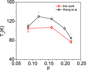
Figure 5. Doping dependence of upper critical temperature Tv determined from Nernst signals. The red open diamond are data of Bi-2212 in this work. The black open hexagons are data determined by Wang et al [5], and are used for comparison.
Download figure:
Standard image High-resolution imageIn OP Bi-2201, Bp is found to be more precise than what is determined from ρ, varying only  from RE and FT. The resulted uncertainty of Bp is around ±10% for all samples, as shown in table 2. This reliability of Bp is due to the clear existence of the TAFF regime in OV Bi-2212, OP and OV Bi-2201, as shown in figure 4. On the other hand, the data at low temperature in UD Bi-2201, UD and OP Bi-2212 are lacking, Bp in these samples requires further investigation.
B0 in Bi-2212 is found to be bigger than in Bi-2201, which is an interesting feature to be explored. It implies that the damping force of impurity scattering is stronger in Bi-2212, for which a qualitative explanation is proposed as follows. As explained in section 2.3.1, damping contributed by impurity scattering can be expressed by resistivity of impurity scattering of the holes inside vortex core, i.e.,  . Based on Drude model of
  , one finds:
  , where τ is the relaxation time. Since nh and
  are significantly bigger in Bi-2212 than in Bi-2201, the higher B0 or damping in Bi-2212 is expected, although a quantitative understanding requires a more careful estimate of τ which is also sample-dependent.
The determination of b in various samples under different doping is made for the first time. In Bi-2201 and Bi-2212, b decreases monotonically from 0.672 to 0.310, and 0.490 to 0.181 respectively, with increasing doping. The uncertainties of b in UD Bi-2212, UD and OP Bi-2201 are around ±11%, for which the determination of b is reliable. On the other hand, for OV Bi-2201, OP and OV Bi-2212, the uncertainties of b are bigger (around  ), due to the fact that the signals above Tc are too small. However, since the result b = 0.186 ± 0.066 in OP Bi-2212 is very close to the results determined from magnetoresistance: 0.183 in Bi-2212 (
 K) [54], we consider that the estimates are reliable.
3.1.3. Comparison to Gaussian fluctuations
The identification of the dominant component of Nernst effect slightly above Tc is important to clarify the physics in pseudogap phase. In this section, we carry out a comparison between Gaussian theory and the present vortex-fluid model, and conclude that the Gaussian fluctuations can not be, but the vortex fluid is the dominant contribution to Nernst signal in Bi-based cuprates.
First, let us carry out an estimate of the thermoelectric coefficient  in 2D system using our vortex Nernst model equation (14). Taking the same η as in magnetoresistance equation (13), we obtain

In addition, we make an assumption that ns decays linearly from  (at zero temperature) to zero (at Tv), i.e.,
  .
.
The comparison is made with the data (red open circles) at low field (B = 1 T) and above  K of (nearly) OP Bi-2212 measured by Ri et al [51]; figure 6 shows a precise agreement between the prediction (red solid line) of the present vortex-fluid model and data at
  . Note that every parameter is determined independently:
  K is determined from the onset temperature of B dependence of magnetoresistance, and
  T is estimated from
  with the coherence length determined as in [5],
  is determined with data of
  at Tc, and
  is determined from the T dependence above Tc. Note that an extra confirmation of the vortex-fluid model in Bi-2212 was obtained in Ginzburg–Landau–Lawrence–Doniach study of diamagnetism, where a mean field of order parameters was introduced to revise the discrepancy between Gaussian theory and data [59].

Figure 6. Temperature dependence of  : comparison to vortex-fluid model and Gaussian-fluctuations theory. Open circles show the data in nearly OP Bi-2212(
 K) at B = 1 T [51]. The solid line is the prediction of vortex-fluid model, equation (17) with
  K,
K,  T,
T,  = nh/2 and b = 0.53. The other two lines are the predictions of Gaussian fluctuations model equation (17), with
  T (dashed line) and
  T (dashed dot line), respectively.
Download figure:
Standard image High-resolution imageOn the other hand, in the limit of  , for 2D superconductors, Gaussian-fluctuation theory predicts
  as [16]

Previously, equation (17) was claimed to agree with data in NbSi (conventional superconductor) [16, 17], OV LSCO (hole doped) [8], UD Eu-LSCO (hole doped) [9] and PCCO (electron doped) [18]. We have made a quantitative comparison between the fitting parameter  from Gaussian-fluctuation theory and low temperature
  measured in those samples. It turns out that the ratio
  is 1.8 for nearly OP (p = 0.15) PCCO, 1.9 for OV (p = 0.17) LSCO, 2.8 for NbSi, 0.25 for UD (p = 0.12) LSCO and 14 for UD (p = 0.11) Eu-LSCO. While the first three measured upper critical fields are slightly below the predicted one, the last two (UD LSCO and UD Eu-LSCO) shows a considerable departure.
This result can be interpreted as following. Since coherence length in conventional superconductors (e.g., NbSi) and electron-doped cuprate (e.g., PCCO) are large, signal above Tc in these samples is dominated by Gaussian fluctuations. However, signals due to Gaussian fluctuations must be smaller in hole-doped cuprates due to their smaller coherence lengths, and thus the contribution of phase fluctuations may not be neglected. Indeed, in OV LSCO, experimental signals are smaller, as consistent with Gaussian-fluctuation theory [8]. On the other hand, in UD samples, strong phase fluctuations result in a larger  . So, Gaussian-fluctuation theory generally underestimates the signal in UD samples (e.g., UD LSCO) [8]. Surprisingly, Gaussian-fluctuation theory overestimates the signal in Eu-LSCO, indicating that the theory predicting only the dependence on coherence length is too simplified, with some physics left over in strong stripe order [15]. In summary, in hole-doped cuprates, Gaussian-fluctuation theory is incapable to describe the UD samples, despite its successful application in OV samples.
Furthermore, we consider the application of equation (17) in Bi-cuprates, e.g. taking Bi-2212 specifically. In figure 6, the black dash line is predicted by Gaussian model with  T, which only describe the data in
  , but significantly higher outside that range. Unfortunately, the fitting value (
 T) is far from being reasonable, since it is much smaller than the estimate from
  T with ξ measured with STM [60]. If the physical parameter
  T is used, the Gaussian theory's prediction (see, the blue dash dot line in figure 6) is much lower than the data. Note that previously, the Gaussian-fluctuation theory of diamagnetism for (nearly) OP Bi-2212 also yields unreasonable fitting parameter (e.g.,
  T) and irrational B dependence [61, 62]. We thus conclude that Gaussian fluctuation alone is unable to describe the physics in pseudogap state, at lest for Bi-based cuprates, for which the phase fluctuations are dominant.
3.2. Unconventional properties of vortex fluid
Unconventional properties of vortex fluid in pseudogap state raise an important issue in HTSC study. Our vortex-fluid model of Nernst effect enables us to determine physical parameters, including local superfluid density, upper critical field and thermal vortex density. These parameter values deliver important information about the physics of pseudogap state, e.g., whether Cooper pairs and vortex survive above Tc (i.e., finite local superfluid density), and how large is the core size (i.e., finite upper critical field), and how thermal vortices density varies with temperature and doping. The properties illustrated through the present phenomenological consideration provide important guide for the further study by microscopic theory to account for quantitative effect of strong phase fluctuations and short range coherence in pseudogap state.
3.2.1. Local superfluid density
Anderson pointed out that, in a vortex fluid, 'ns is not the conventional macroscopic quantity giving the penetration depth, which is its average over phase fluctuations, but is defined microscopically...' [25]. Indeed, in the BKT scenario of 2D superconductor, thermal vortices emerge above Tc and results in a dramatic increase of the penetration depth [63] and the macroscopic quantity of  (see, open hexagon in figure 7) quickly decreases to zero. However, the local superfluid density which flows within interstitial puddles between vortex cores remains finite, which can induce a vortex Nernst effect. An advantage of the present vortex-fluid model is to allow one to determine the local superfluid density from Nernst signal, and then discuss its unconventional temperature dependence in pseudogap state.
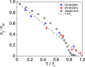
Figure 7. The normalized superfluid density  versus
  determined in this work for OV Bi-2201 (
 = 0.681
  cm−2) and OV Bi-2212 (
 = 9.71
  cm−2), where
  is shown in table 3. A linear law
  is obtained. The open and black hexagons are the data
  derived from microwave penetration depth in OP Bi-2212 (
 K,
K,  cm−2) with
  K [63].
Download figure:
Standard image High-resolution imageEquation (15) yields an expression for the local superfluid density  :
:

where  = 24.6 Å for Bi-2201, 30.9 Å for Bi-2212. In order to extract
  ,
,  should be estimated. Since ρ for the samples corresponding to the present Nernst data is not available in literature,
  needs to be estimated from ρ of other (similar) samples with the same Tcs. According to equation (13),
  is also the resistivity of holes in normal fluid. Based on the Drude model of normal metal, the conductivity is proportional to hole concentration p, thus

Hence,  can be determined for each sample, once a value of
  at some doping is obtained. The results are shown in table 3, using the data
  mΩ cm in OP (p = 0.16)
  [50] and
  mΩ cm in the OV (p = 0.24) Bi-2201 [64].
Table 3.
Characteristic resistivity  estimated with equation (19).
| Sample | UD Bi-2201 | OP Bi-2201 | OV Bi-2201 | UD Bi-2212 | OP Bi-2212 | OV Bi-2212 |
|---|---|---|---|---|---|---|
 (mΩ cm) (mΩ cm) |
0.41 | 0.20 | 0.15 | 0.19 | 0.11 | 0.076 |
In this work, we find that local superfluid density indeed exhibits interesting behaviors. As shown in figure 7,  of OV Bi-2201 and OV Bi-2212 determined from equation (18) nearly collapse on a straight line
  , where
  is a fitting parameter. Two distinct features different from the temperature dependence of macroscopic superfluid density (see, open hexagon in figure 7) are noteworthy: a finite ns above Tc and a universal linear temperature dependence below Tv. The finite ns above Tc and vanishing of ns at Tv but not Tc is very indicative of the nature of pseudogap state: full of thermal vortices. This indicates that the thermal effects above Tc and below Tv are restricted within the vortex core, perhaps in the form of qp holes, while a local superfluid around the (thermal) vortex core still survives. Note that a linear T dependence of ns at low temperature has been widely observed in HTSC [65] and can be described by the standard BCS theory of d-wave superconductor; but the presently observed linear behavior of local superfluid density above Tc is exotic, and requires further theoretical explanation. For more discussion, see section 3.2.4.
Strictly speaking, the concentration of oxygen deficiency in the CuO2 plane are different in each sample so there exists a certain deviation of this estimated  , and hence of ns [64]. However, the relative values of ns with respect to temperature are considered to be reliable.
3.2.2. Upper critical field
Upper critical field  represents a crossover from a vortex fluid to the normal state due to overlap of magnetic vortex cores, and it is also a probe of the coherence length ξ because
  . Since core–core collisions are enhanced with increasing magnetic field (see, equation (13)) in cuprate HTSC, magnetoresistance presents a 'knee' behavior, instead of following a Bardeen–Stephen law [5, 42, 53]. Therefore, one can no longer make an exact definition for
  from magnetoresistance as in conventional superconductor. Indeed, empirically determined '
 ' from the 'knee' feature (see crosses in figure 8(a)) displays a sharply different behavior from that described by the conventional Werthamer–Helfand–Hohenberg (WHH) theory for BCS superconductors [66]. Recently, distinct progress has been achieved using Nernst signal [5, 55] and diamagnetism [67, 68], in which
  is defined as the field where eN and M versus B extrapolates to zero. Our model enables one to make this determination in a wider range of T and B, since it may be considered as a more sophisticated version of the simple method by Wang et al, especially when the measured profile is imperfect.

Figure 8. Temperature dependence of  determined from eN via equation (14) in OP Bi-2212 (a) [55, 56] and OP and OV Bi-2201 (b) [5].
  in nearly OP Bi-2212 determined from magnetoresistance (ρ equals 90% of the normal-state resistivity) [66] are shown by black crosses for comparison.
Download figure:
Standard image High-resolution imageThe T dependence of  (see, section A.2) as shown in figure 8 displays a slow variation near Tc, consistent with the results of linear extrapolation of Nernst and diamagnetism versus B [5, 68]. For instance, at T = 5–40 K in OP Bi-2201 (or T = 70–100 K in OP Bi-2212),
  is presently in [43.3, 54.2] T (or [40.3, 81.8] T), as compared to [42, 52] T (or [43, 90] T) according to extrapolations of Nernst or diamagnetism [5, 68]. This behavior of finite
  above Tc is different from the canonical BCS behavior described by WHH theory, in which
  at Tc due to gap-closing. If
  above Tc in Bi-based cuprates, the strong and positive eN above Tc in OP Bi-2212 must be interpreted by Gaussian fluctuations which is shown above (in section 3.1.3) to be unsuccessful, and the linear decaying of eN in high-field in OP Bi-2201 cannot be explained by the logarithmic decay of Gaussian fluctuations. Furthermore, the finite
 also implies finite core size or coherence length ξ, which has a weak T dependence near Tc. This is highly consistent with the Pippard coherence length
  determined from gap amplitude
  which is also observed to be finite and varies slowly above Tc in ARPES measurement [69]. In conclusion, the finite
  above Tc is physically sound in Bi-based cuprates, indicating that vortices with finite core size survive above Tc.
On the other hand, in figure 8(b), anomalous increase of  with increasing temperature occurs above Tc in OV Bi-2201, which might be the evidence of the contribution of amplitude fluctuations. The signal above Tc is one order of magnitude lower than the maximum signal at low temperature, thus can be influenced by weak amplitude fluctuations tail [5], leading to an overestimate of
  . In addition, for extremely UD samples, anomalous increase of
  is also present at T near and above Tc. A possible interpretation is exotic qp excitation due to density-wave order in this regime [12]. While the regular behaviors of
  in most regimes ensure the validity of the vortex-fluid model, the irregular behaviors of
  deduced with vortex fluid model provide a sensitive probe for additional contributions of qp or amplitude fluctuations. The present study thus serves a basis for developing a more comprehensive theory in the future.
3.2.3. Thermal vortex density
Equation (3) is able to predict the temperature dependence of thermal vortex density  , as shown in figure 9(a). Note that
  in UD sample is much larger than in OP and OV samples, in both Bi-2201 and Bi-2212. We argue that the energy cost to excite a thermal vortex-antivortex pair is proportional to ns. Thus, thermal vortex is easier to be excited in UD sample. Furthermore, it is interesting to observe a similar temperature dependence for each sample. In figure 9(b), normalized densities
 ![${n}_{T}/{n}_{T}{({T}_{v})=\exp [-2b({T}_{v}/{T}_{{\rm{c}}}-1)}^{-1/2}({t}^{{\prime} -1/2}-1)]$](https://content.cld.iop.org/journals/1367-2630/19/11/113028/revision2/njpaa8ceeieqn173.gif) collapse into three groups, where
collapse into three groups, where  is the maximum density at Tv and
  . The difference is controlled by one material parameters
  which may be treated as a normalized coherence strength to resist thermal vortex activation. For Bi-2212,
  is nearly doping independent with Sc ranging from 0.42 to 0.47, indicating a universal normalized resistance of thermal vortex activation for different doping of Bi-2212. For Bi-2201, however, two behaviors of
  appear, one in UD and OV sample with
  , indicating that the normalized coherence strength in bilayer system is stronger than in monolayer bilayer system. But, an exception is found for OP Bi-2201 that Sc reaches a maximum (i.e., 0.55) with a strong decline of
  this last observation requires further theoretical explanation.

Figure 9. Thermal vortex density  versus T in Bi-2201 and Bi-2212. (a)
 ![${n}_{T}={({B}_{l}/{\phi }_{0})\exp [-2b(T/{T}_{{\rm{c}}}-1)}^{-1/2}]$](https://content.cld.iop.org/journals/1367-2630/19/11/113028/revision2/njpaa8ceeieqn182.gif) are calculated with parameters in table 2, and plotted in various lines and colors. (b) Normalized density
are calculated with parameters in table 2, and plotted in various lines and colors. (b) Normalized density ![${n}_{T}/{n}_{T}{({T}_{v})=\exp [-2b({T}_{v}/{T}_{{\rm{c}}}-1)}^{-1/2}({t}^{{\prime} -1/2}-1)]$](https://content.cld.iop.org/journals/1367-2630/19/11/113028/revision2/njpaa8ceeieqn183.gif) of each sample in (a), where
of each sample in (a), where  is the maximum density at Tv and
  .
.
Download figure:
Standard image High-resolution image3.2.4. Vanishing of short-range phase coherence
In the BKT scenario, long range phase coherence is destroyed by the proliferation of thermal vortices. Here, the quantification of the Nernst signal allows us to examine the dynamical properties of thermal vortices, and to propose a mechanism for the vanishing of short-range phase coherence, namely the lifetime of thermal vortices versus the cycle period of Cooper pairs around the core, as we explain now.
For a vortex, short-range phase coherence can be quantified by the cycle period of Cooper pairs around the core, i.e.,  . This coherence may be destroyed by the activation and annihilation of thermal vortices, whose characteristic time defines the average lifetime of thermal vortices (or coherence time) during which the local wavefunction becomes totally dephased. This lifetime can be estimated by
  , where sv is the moving path length of the thermal vortex during its lifetime, determined by
  , the perimeter of a circle with diameter
  , and vR is the random velocity of the vortex. The latter can be obtained by an energy estimate [26] due to quantum fluctuations of holes inside vortex core,
  . It follows that
  , and the ratio of the two time scales is

Now, we argue that vanishing of short-range phase coherence requires that  equal to 1 at the upper critical temperature Tv. Using the parameters near Tv, we can obtain
  = 1.13 ± 0.07, 0.91 ± 0.10 and 0.98 ± 0.30 for three samples, OP Bi-2201, OP Bi-2212 and OV Bi-2212, respectively. For other samples,
  at Tv is either unavailable or is unreliable due to too big errors. Thus, we consider that available data confirm our proposal. Physically, the near unity is originated from the key fact that motions of thermal vortices and Cooper pairs near the core both depend on the same core size ξ.
Furthermore, we speculate that this understanding may also help in interpreting the temperature dependence of ns. This is because that the lifetime for a vortex (magnetic or thermal) can be defined as  . When temperature increases, both
  and ns decays. If we assumed that the decay of ns is induced by the dephasing effect of vortex activation and annihilation, a simple relation, i.e.,
  can be obtained, where
  is the superfluid density at zero temperature. At zero temperature,
  is infinite thus
  . While at Tv, ns vanishes. This interesting idea will be explored elsewhere in the future.
4. Discussion and conclusion
4.1. Application to other HTSC
In the present work, we have developed a systematic procedure to analyzing the effect of vortex dynamics embedded in magnetoresistance ρ and Nernst signal eN, and this procedure is applicable to other extremely type-II layered superconductor. Once ρ and eN data of a new sample are available, the RE can be conducted first using asymptotic analysis at large and small limits of T and B. Note that for electron-doped cuprates, some UD hole-doped cuprates [9], and even iron-based superconductor [70], the contributions of qp should be subtracted with a linear or nearly linear model [5, 57]. The procedure of RE can be summarized as following. Step one, intuitively estimate the upper critical temperature Tv and characteristic resistivity  from the convergent (or saturated) regime of ρ. Step two, carry out a magnitude analysis of the maximum eN signal with equation (15), and predict the characteristic superfluid density
  if the carrier effective mass is available (e.g., for

 ,
,  me [70]). The comparison between
  and carrier density in the sample allows one to judge the validity of the vortex-fluid scenario. Step three, determine
  (thus Bl) from the linear extrapolation of eN in strong fields according to equation (A7). Sometimes, linear regime of eN in strong fields is not measured (e.g., for

 [70]), then use the values from other measurements of similar sample [71] such that the determination of ns in the final step can be achieved. Step four, use the data at low T of ρ (or eN) (with significant pinning effect) to determine Bp with equation (A2) (or equation (A9)). Step five, determine B0 from the linear field dependence of ρ or eN in low fields at Tc. Step six, determine the Kosterlitz coefficient b from the sharp increase near Tc of ρ in zero field with equation (3). Finally, estimate the T-dependent local superfluid density ns by the calculation of the peak of eN versus B with equations (A12) and (18). By the way, although it is better to obtain measurements of magnetoresistance and Nernst signal simultaneously and in wide T and B range, there are other ways to complement the data from the literatures using our vortex-fluid model. Details of the above procedure are presented in the appendix.
4.2. Validity of entropy model
It is important to discuss the validity of the entropy model, i.e., equation (6), which is similar to Anderson's original proposal [29], but is more general. Although it appears that equation (6) is an extension of the BKT scenario, but we argue that in a dense vortex fluid of 2D superconductor, the fluctuations are strong, so that the probability of proliferation of (magnetic or thermal) vortices is substantial, and the balance equation equation (6) is approximately valid. Quantitatively, the current description of Bi-2212 [51], equation (6) (with a relative mean square root error equals 0.37) is more precise than the Maki's model deduced form TDGL near  (with a relative mean square root error equals 0.58) [72]. Thus, equation (6) is a reasonable approximation (which is in fact the most precise one for Bi-2212 so far) of transport entropy in Bi-cuprates, despite its simplicity.
Strictly speaking, equation (6) is not valid at low temperature where ordered motions dominate so that heat in vortex is much smaller than the kinetic energy of supercurrents. In this case, an energy transformation mechanism between ordered and disordered motions may take place, and the ratio  needs to be multiplied by a factor which increases from zero (at zero temperature) to a finite value at high temperature. This extension is beyond the scope of the present work, and will be considered in the future.
4.3. Effects of fluctuating vortices
In previous studies, vortex motions are believed to originate only from phase fluctuations while amplitude is frozen, implying that amplitude fluctuations play no role in vortex fluids [7]. Here, we argue, based on an estimate below of the lifetime  of fluctuating Cooper pairs [73], that magnetic field can also drive fluctuating vortex pairs. In fact, a dimensional estimate of
  yields that
  , while the cycle period of the fluctuating pair near the core is
  . In overdoped samples (due to small ξ), one finds that
  , e.g.,
  in OV Bi-2201 (Tc = 22 K), which implies that a group of fluctuating Cooper pairs can form a fluctuating vortex in about a half cycle period. The total heat and charge transport, thus the Nernst signal, must be a superposition of the contribution of conventional vortices and fluctuating vortices. Therefore, we can transform the Gaussian fluctuations model
  to a fluctuating vortex-fluid model
  , where
  is the transport entropy of fluctuating vortices,

Following equation (21), we introduce an integrated entropy model of conventional vortices and fluctuating vortices  , where
  is the contribution of conventional vortices. In UD samples where phase fluctuations dominate, the fluid is composed of conventional vortices; while in extremely OV samples, the fluctuating vortices play a important role. Thus, this integrated model may sets a basis to describe the intermediate regime of phase and amplitude fluctuations.
4.4. Conclusion
In order to describe the Nernst effect in pseudogap state, many insightful ideas have been proposed, including vortex tangles [25] and qp associated with a density wave order [10]. However, the signal's dependence on T and B is complicated, due to multiple components and mechanisms in play, and hence has not yet been addressed quantitatively. The present phenomenological model takes upon this challenge, and provides a completely analytical description for the dominant vortex component, which covers several phase regimes and involves several relevant processes such as thermal and magnetic vortex activation, impurity scattering, core–core collisions and pinning.
The main conclusion of the work is that both magnetoresistance and Nernst signal in Bi-based samples are accurately described by vortex-fluid model at low and high fields and below and above Tc, which quantitatively confirms the indispensability of vortex fluid and phase fluctuations in pseudogap state. The model quantifies the unconventional vortex properties by local superfluid density, upper critical field and thermal vortices density, which adds quantitative contents to discuss the nature of pseudogap. The fully analytic nature of the model enables the signal separation of vortex and non-vortex components, thus represents the first step towards achieving a comprehensive theory of Nernst effect for all HTSC, by integrating multiple components. Furthermore, the model provides an opportunity to comparing the physical properties of Fe-based to cuprates HTSC according to the temperature, doping and layer dependence of parameters.
Acknowledgments
We thank L Yin for many constructive discussion during the early stage of this work. We thank Y Wang for a very helpful discussion. This work is partially supported by National Nature Science (China) Fund 11452002.
Appendix.: Parameters determination
A key result of the present work is to demonstrate that it is possible to derive reliably the values of the model parameters, as we show below.
The determination of model parameters is conducted in two steps. The fist step is a rough estimation (RE), using asymptotic analysis at high and low limits of T and B, where naturally one or two leading mechanisms are dominant. In this case, only one or two parameters appear, so their approximate values can be obtained. This determination is approximate because empirical data do not go very far in the asymptotic limits; more often the effects of variation of the multiple parameters are entangled together, so that a global optimization is necessary to find more accurate description of data. This is then accomplished by the second step of fine tuning, which define the best set of parameter values by minimizing the error between the predictions and empirical data. In other words, the parameters are tuned around the roughly estimated values to achieve a better fitting of a set of data (multi-curves).
The fine tuning (FT) is realized by a least square fitting process. For example, in the determination with Nernst signal, we divide the entire set of parameters into groups so that the FT can be conducted one group after another, with the former results substituted into the later calculation. This iterative process runs until a local minimum of the error is reached. If there are more than one local minimums, a comparison between them decides the global minimum, and then the FT ends with a set of precisely determined parameters. Sometimes, the physically optimal point is not the global minimum but the local minimum. Therefore, to determine the local minimum, we need to define the range of parameters to be explored, to be specified in the main text.
The reliability of the parameters depends on the precision of the comparison between predictions and the data, and the uncertainties of the parameters. The later can be expressed by error bar. Once the optimal set of parameters are obtained, the error bar is determined once the upper boundary of the RMSE between the predictions and empirical data reaches a threshold equals to the measurement uncertainty.
A.1. Determine parameters with flux-flow resistivity
In the resistivity model equation (13), there are seven parameters, namely Tc,  , Tv, B0, Bp, Bl and b, to be determined by experimental data. Tc can be easily estimated from the transition temperature of zero resistivity. In this section, we explain how other parameters are determined, using magnetoresistance data of optimally doped (
 )
)  [50].
[50].
A.1.1. Rough estimate
First, let us discuss the RE. In section 2.1, we assume that the high T limit of thermal vortex density is as dense as magnetic vortices at  , thus
  .
.  can be estimated as
  . Thus,
  T as
T as  Å is measured by STM [60].
Near Tv, core–core collisions are dominant in η since the density of thermal vortices is dense, thus B0 can be neglected. Then, ρ can be expressed as

which predicts that ρ increases with B for  and converge to
  for T approaching Tv. We use the convergent regime of the experimental curves (see figure 3) to carry out a RE of Tv and
  . The convergent regime corresponds to the range where the curves at the highest (17.5 T) and lowest (0) become close (or overlapped). In practice, we consider the overlap starts where the difference of the two curves equals the scatters of each curve, which is about 5
  cm. Applying this criteria, we obtain
 ![${T}_{v}\in [104,120]$](https://content.cld.iop.org/journals/1367-2630/19/11/113028/revision2/njpaa8ceeieqn238.gif) K and
K and ![${\rho }_{0}\in [0.098,0.133]$](https://content.cld.iop.org/journals/1367-2630/19/11/113028/revision2/njpaa8ceeieqn239.gif) mΩ cm. The middle values, e.g.,
mΩ cm. The middle values, e.g.,  K and
K and  mΩ cm, are taken to be the roughly estimated values.
Bp is determined from the low T limit (i.e., the TAFF regime) of the resistivity profiles. At  , pinning effect dominates and B0 is neglected. We define
  ,
,  , then a linear formula is obtained,

where  , and b0 contains the contributions from B0 and data error. A least square fitting of the line yields
  so that
  T, as shown in figure 10.

Figure 10. Linear fitting of  versus
  at B = 9 T. The red open stars are the data of
  . The black dash line is the linear fitting curve. The blue open squares are the data of ρ.
Download figure:
Standard image High-resolution imageB0 is supposed to dominate in low fields where vortices flow individually in materials with weak pinning. However, for  [50], the melting field
  T indicates a significant pinning effect, thus B0 is nearly invisible at low temperature. The contribution of core–core collisions and pinning effect is presented by f,

To suppress this contribution and avoid the effect of thermal vortices, we propose to determine B0 at Tc and near H', where H' is the minimum of f at Tc. At Tc, the equation (13) is simplified to

Since Tv and Bp are determined, the minimum of f is found to be  = 4.7 T at
  T. According to calculation, f is approximately a constant near
  , thus the data at
  (
(
 cm) and 1 T (
 cm) are used in the linear fitting. Finally,
  T is obtained.
b is determined near and above Tc with Kosterlitz model [37]. At  , we have the following relation:

where i = a, b. Equaling the case a and b, we obtain BT. BT calculated from  T and
T and  T in the range
 ![$T\in [90,100]$](https://content.cld.iop.org/journals/1367-2630/19/11/113028/revision2/njpaa8ceeieqn265.gif) K is shown in figure 11. According to equation (3), the Kosterlitz coefficient
K is shown in figure 11. According to equation (3), the Kosterlitz coefficient  is fitted from the data at
 ![$T\in [90,94]$](https://content.cld.iop.org/journals/1367-2630/19/11/113028/revision2/njpaa8ceeieqn267.gif) K.
K.

Figure 11. Determination of b from the fit (blue dashed line) of BT (red symbols) based on Kosterlitz model equation (3).
Download figure:
Standard image High-resolution imageA.1.2. Fine tuning
In this step, we vary the five parameters ( , Tv, B0, Bp and b) around their roughly estimated values to get a precise fitting of the experimental curves, while keeping
  T unchanged, following the argument in the beginning of this section. This fine tuning process needs to set up a ranges for each parameter. First, the result of RE already yields
 ![${T}_{v}\in [104,120]$](https://content.cld.iop.org/journals/1367-2630/19/11/113028/revision2/njpaa8ceeieqn270.gif) K and
K and ![${\rho }_{0}\in [0.098,0.133]$](https://content.cld.iop.org/journals/1367-2630/19/11/113028/revision2/njpaa8ceeieqn271.gif) mΩ cm. Secondly, B0, Bp and b are set to be positive, as it is evident from their physical meaning. Then, we treat the empirical data of five curves at H = 0, 0.5, 3, 9 and 17.5 T for
mΩ cm. Secondly, B0, Bp and b are set to be positive, as it is evident from their physical meaning. Then, we treat the empirical data of five curves at H = 0, 0.5, 3, 9 and 17.5 T for  K as an ensemble, and evaluate the RMSE of the predictions from the data, when the five parameters vary in the range specified. Finally, the smallest RMSE ≈ 3.5
  cm is reached and the fitting is shown in figure 3.
According to the procedure introduced in the beginning of this section, the error bar can be determined from the uncertainty of the original data [50], which approaches ±2.5  cm. We thus use 5
  cm as the upper boundary of the RMSE function. The error bar for any one parameter is calculated when the others are set to their FT-determined values, and the results are shown in table 1.
A.2. Determine parameters with Nernst effect
The systematically measured Nernst signal allows us to do reliable parameter determinations. In this part, equation (14) is applied to the six samples in Bi-2201 and Bi-2212 [5, 52, 56]. The process of parameters determination with eN is similar to the one with ρ but there are some more steps due to the two more T dependent parameters  and
and  . In the following, OP Bi-2201 is taken as an example to show the specific procedures.
A.2.1. Rough estimate
In RE, the asymptotic analysis at high and low limits of T and B is also the key strategy. Tv can be determined from the zero point of the linear extrapolation of the peak at very high temperature. Using similar linear extrapolation in high fields,  is obtained.
  and Bp can be determined from field dependence of the signal in the TAFF regime. The nearly linear field dependence of eN near the minimum of f below and near Tc can be used to determine B0. Meanwhile, b can be determined from the peaks of the profiles above Tc.
On the profile of  versus B, when
  ,
,

Since ns approaches 0 at Tv, the peak  of the profile approaches zero. Since
  versus T is a nonlinear curve at large T range, only the data (50 and 65 K) nearest to zero are used in the linear extrapolation, shown in figure 12(a). Finally,
  K is obtained. The uncertainty of the data is estimated to be ±100 nV K−1 (discussed in the end of this section), and the error bar of Tv is found to be ±6.2, thus
  K.
K.
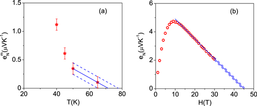
Figure 12. Linear extrapolation to determine  and
and  in OP Bi-2201. (a) Linear extrapolations (blue solid line) of
  at 50 and 60 K to determine
  . The blue dashed line represents the error bar of extrapolation. (b) Linear extrapolations (blue solid line) of eN in high fields to determine
  .
.
Download figure:
Standard image High-resolution imageWhen  , a linear dependence of B can be obtained from equation (14),

 represents the zero point of the signal. In figure 12(b), a linear extrapolation of the high fields data, applied to the curve at 20 K, yields
  T. Results of
  at other temperatures are shown in table 4. Since
  (Tc = 28 K),
  can be estimated as
  (30 K) = 48 T.
Table 4.
 determined from linear extrapolation of eN.
| T (K) | 5 | 11 | 20 | 30 | 40 |
|---|---|---|---|---|---|
 (T) (T) |
50.0 ± 3.3 | 45.0 ± 1 | 45.0 ± 0.7 | 48.0 ± 1.3 | 50.0 ± 3.6 |
At low temperature and fields (i.e., the TAFF regime), pinning effect is dominant in damping viscosity. Thus, B0 can be neglected in eN,

Taking the logarithm of the two sides of eN in equation (A8), we can obtain

where ![$y={\rm{ln}}[{\rm{ln}}({H}_{{\rm{c}}2}/B)]-{\rm{ln}}{e}_{N}$](https://content.cld.iop.org/journals/1367-2630/19/11/113028/revision2/njpaa8ceeieqn300.gif) ,
,  ,
,  ,
,  . The linear fitting of the data allows us to determine the parameters,

The fitting at T = 20 K is shown in figure 13, and  T,
T,  μV K−1 are obtained. Data in very low fields are not used because the signals are very weak thus the relative error are big.

Figure 13. Linear fitting of ![${\rm{ln}}[{\rm{ln}}({H}_{{\rm{c}}2}/B)]-{\rm{ln}}{e}_{N}$](https://content.cld.iop.org/journals/1367-2630/19/11/113028/revision2/njpaa8ceeieqn306.gif) versus
versus  to determine
  and
and  at T = 20 K.
Download figure:
Standard image High-resolution imageA nearly linear equation can be obtained from the model equation (14) of the Nernst effect at the minimum of f and below Tc,

where ![$g={e}_{N}/[{e}_{T}\mathrm{ln}({H}_{{\rm{c}}2}/B)]$](https://content.cld.iop.org/journals/1367-2630/19/11/113028/revision2/njpaa8ceeieqn310.gif) . Similar to equation (A4), the data in low fields and high temperature should be used to determine B0. In figure 14(a), g versus B at T = 20 K shows a linear regime in low fields (from 1 to 8 T), which supports a linear fit (
. Similar to equation (A4), the data in low fields and high temperature should be used to determine B0. In figure 14(a), g versus B at T = 20 K shows a linear regime in low fields (from 1 to 8 T), which supports a linear fit ( ). But the minimum of f is so big (31.1 T) that B0 is found to be very small (0.1 T). In addition, the error of the slope yields that B0 varies in ±1 T. Thus, B0 can be reasonably chosen as 0.
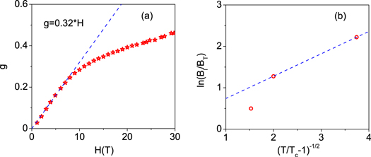
Figure 14. Linear fitting to determine B0 and b in OP Bi-2201. (a) Linear fitting ( , blue solid line) at the minimum of f (equation (A3), red symbols) versus H. (b) Linear fitting (blue dashed line) of
  versus
  near
near  K at 30 and 35 K.
Download figure:
Standard image High-resolution image
Since  T is estimated, b can be determined from the peak value
  above Tc, where

BT can be calculated from this formula directly. According to Korsterlitz model equation (3), a linear model can be obtained as

where  ,
,  ,
,  and b2 contains the errors. b can be determined from the linear fit of equation (A13). In figure 14(b), the data near Tc (30 and 35 K) are used to conduct the linear fitting and
  is obtained. The results of RE are shown in table 2.
A.2.2. Fine tuning
Since both eT and  in equation (14) are T-dependent, the FT procedure of the Nernst effect is a little more complicated, which requires to run an iteration program. First, the parameters are divided into two groups. One group is made up of intrinsic parameters B0, Bp, Bl, b and Tv. The other contains the T-dependent parameters
  and
and  . The RE helps to define the ranges of the fitting parameters, e.g.,
 ![${T}_{v}\in [65.3,77.7]$](https://content.cld.iop.org/journals/1367-2630/19/11/113028/revision2/njpaa8ceeieqn325.gif) K,
K, ![${H}_{{\rm{c}}2}\in [44,53.6]$](https://content.cld.iop.org/journals/1367-2630/19/11/113028/revision2/njpaa8ceeieqn326.gif) T,
T, ![${B}_{l}\in [46.7,49.3]$](https://content.cld.iop.org/journals/1367-2630/19/11/113028/revision2/njpaa8ceeieqn327.gif) T and
T and  . Besides,
  ,
,  and
and  are set to be constraints. Second, we treat the empirical data of five curves at T = 5, 11, 20, 30 and 40 K for
  T as an ensemble. Using the iteration program, the FT can be conducted, one group after another, with the former results substituted into the later calculation. This iterative process runs until a local minimum (RMSE ≈ 0.0993 μV K−1) in the parameter space specified as above is reached.
In the Nernst experiment [5], the error of the voltage measured by nanovoltmeter is ±5 nV, thus the uncertainty of the Nernst signal  is estimated to be ±25 nV K−1. By private communication, Y. Wang indicates that the noise in strong fields should be larger, thus
  is larger than ±50 nVK−1 (the maximum value may be ±0.1 μV K−1 at 45 T), consistent with the typical fluctuations of the data. In the present work, only data below 30 T are used. We choose a rational fitting error of ±100 nV K−1 as the upper boundary of the error function for the samples except for UD Bi-2201. For UD Bi-2201, the local minimum error is 0.152 μV K−1, thus we set 0.2 μV K−1 as the upper boundary, to reveal the sensitivity of the model. The procedure to determine the error bar is similar to that above for ρ, except Bl is assumed as equals to
  at Tc (with error bar). The final results of FT are shown in table 2 and the multi-curves fitting figure is shown in figure 4(b).