


Abstract
We investigate an extension of the quantum Ising (QI) model in one spatial dimension including long-range  interactions in its statics and dynamics with possible applications from heteronuclear polar molecules in optical lattices to trapped ions described by two-state spin systems. We introduce the statics of the system via both numerical techniques with finite size and infinite size matrix product states (MPSs) and a theoretical approaches using a truncated Jordan–Wigner transformation for the ferromagnetic and antiferromagnetic case and show that finite size effects have a crucial role shifting the quantum critical point of the external field by fifteen percent between thirty-two and around five-hundred spins. We numerically study the Kibble–Zurek hypothesis in the long-range QI model with MPSs. A linear quench of the external field through the quantum critical point yields a power-law scaling of the defect density as a function of the total quench time. For example, the increase of the defect density is slower for longer-range models and the critical exponent changes by twenty-five percent. Our study emphasizes the importance of such long-range interactions in statics and dynamics that could point to similar phenomena in a different setup of dynamical systems or for other models.
Export citation and abstract BibTeX RIS
1. Introduction
Common quantum many-body models, such as the quantum Ising (QI) model or Hubbard models, include only a nearest-neighbor interaction, while e.g. the Coulomb forces or the dipole–dipole interactions have power law tails of the form  . This leads to the core question: 'To what extent does the physics of these models changes when including decaying long-range interactions?' Physical models with tunable long-range interactions have been successfully realized in recent experiments due to advances in atomic and molecular physics. This especially includes experiments in heteronuclear polar molecules in optical lattices [1, 2] and trapped ions [3]. Further examples for the realization of a long-range Ising model are the cold ion experiment in [4] realizing a two-dimensional lattice and ultracold molecules with long-range dipole interactions, which have been successfully realized in recent experiments [5, 6]. Furthermore, realizations in Rydberg atoms through long-range van der Waals interactions [7, 8] or solid state physics, e.g. based on
  [9], exist and provide a large number of spins, e.g. in comparison to ultracold ion experiments at the current stage. In addition, magnetic dipoles can lead to the same long-range interactions which have been realized in recent experiments in terms of chromium [10], erbium [11], and dysprosium [12], and further setups with long-range interactions tuned by optical cavities have been made [13], too. The list of experiments can be further extended with nitrogen vacancies in diamonds with a ferromagnetic long-range Ising interaction [14]. Recent advances in quantum annealing have fostered the mapping of problems onto a generalized QI model [15], which is a more general Hamiltonian than the long-range interaction. This is as well the case for quantum spin glasses [16]. These systems have in common that they can be described by two-state spin models with
  interactions coupled to external transverse fields, including the long-range quantum Ising (LRQI) model. While the experimental systems range from implementations in one to three-dimensions, we study a one-dimensional system, because our numerical techniques are best suited to this case. The recent work of several groups discussed new emerging phases due to long-range interactions [17] and different regimes that hold or violate the Lieb–Robinson bounds, limiting the speed of transferring information depending on the initial state [18].
For numerical studies of many-body systems, tensor network methods offer a variety of algorithms which can be tailored to certain problems [19]. The infinite matrix product states (iMPSs) [20] on infinite translationally invariant lattices and the matrix product states (MPSs) for finite systems are well suited for the ground state calculations of quantum systems. Dynamics can be simulated with the time-dependent variational principle (TDVP) [21], where other methods as Krylov or local Runge–Kutta were explored for comparison [22, 23]. The QI model is not only fundamental because of the various experimental implementations mentioned, but also since it has a similar classical model in the Ising model, originally introduced in 1925 [24] with analytic solutions in one and two-dimensions. Moreover, the quantum model in d dimensions can be mapped onto the classical Ising model in  dimensions; the solution for the classical model in two-dimensions is linked to our one-dimensional quantum chain. Therefore, it is an ideal starting ground to explore long-range interactions before including them into other models and has always been the toy model to explore a huge variety of methods before using them on other models since it is the description for a vast majority of physical problems. This includes methods such as the exact spectrum, perturbation theory, or the mapping of the ferromagnetic case to the corresponding classical Ising model in higher dimensions without using numerical methods. It is applicable to many problems that can be mapped into two-level systems and therefore accessible for researchers from fields as different as solid state physics and atomic, molecular, optical physics just mentioned before.
While the experimental systems can be in higher dimension, we consider one-dimensional spin chains with long-range interactions subjected to the external magnetic field in its transverse direction. From there, we lay out the discussions of static and dynamic simulations via tensor network methods for models with long-range interactions. Numerical algorithms based on tensor networks perform optimally in one-dimension and have limitations in higher dimension, although they have been proposed for two-dimensional systems [25]. However, the Kibble–Zurek mechanism (KZM) yields a fascinating topic for the LRQI model in real time evolution; for example, quenching across the critical point could be used for state preparation whenever it is easier to prepare the ground state in one phase.
As for the usual QI chain, that is integrable, both static properties such as the phase diagram, critical exponents or correlation lengths, and dynamic properties have been studied at length. The latter includes the KZM being applied to show that the density of defects in the ferromagnetic chain follows a scaling law for linear quenches [26–28], i.e. the density of defects increases for faster quenches across the quantum critical point. Those properties of the Ising model have always paved the road to study other models. Then, there appears a natural question: How do these long-range interactions affect the well-known results in the QI model? These answers are relevant to ultracold molecules with characteristic long-range dipole–dipole interactions or Rydberg atoms with long-range interactions. Therefore, we present the reader new results on the Kibble–Zurek scaling with the comparison of the static results using three different approaches. Our analytical approach uses an approximation which truncates phase terms of the Jordan–Wigner transformation and the two numerical algorithms cover infinite and finite systems. With those comparisons we see finite size effects as the lower critical external fields for decreasing system sizes; dynamic simulations are based on these results. We introduce the dynamics with experimentally measurable observables such as the local magnetization in figure 1 and compare the scaling of defects with the Kibble–Zurek hypothesis. The KZM posits that for decreasing quench times, the defect density increases less for the ferromagnetic case in regard to the nearest-neighbor QI model. In contrast, the number of defects stays at the same rate for the antiferromagnetic model for faster quenches in comparison to the QI model. With the exponent of the KZM changing about 25% in the ferromagnetic case, this should be an observable effect. Apart from the prediction of defects when quenching across the quantum critical point for preparing states it might even allow for characterization of long-range effects according to the critical exponent.
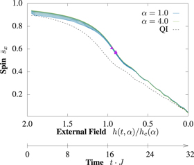
Figure 1. Quench of the long-range quantum Ising model. The mean local x-magnetization as average over the sites of the measurement of  , i.e.,
  , is a typical observable for spin models and realizable in cold ion experiments. The measurement during the quench from the paramagnetic phase to the to the ferromagnetic phase for different interaction strength governed by power law
  displayed for α in steps of 0.2 is compared to the nearest-neighbor quantum Ising (QI, dashed curve). The triangles mark spots with first maximum of the gradient disregarding numerical fluctuations. The magnetization in x-direction is vanishing equally for all α, since the quench is starting at
  and ending at
  .
.  is the value of the quantum critical point which differs for each α. We emphasize the unified dynamics of the quench independent of α for the symmetric setup around the critical point.
Download figure:
Standard image High-resolution imageThroughout the paper we concentrate on both the antiferromagnetic and ferromagnetic case. Moreover, we address the challenges with those studies, e.g. simulations breaking down in certain regimes of the LRQI. We use the open source matrix product states package (OSMPS) [22] freely available from [29]. As a secondary goal, we provide with those practical calculations and discussions on the numerical results a basis for future researchers to interpret their results on statics and dynamics gained with OSMPS or any other tensor network method library. The models suitable for further studies range from more advanced spin models of XYZ-type to all kind of Hubbard models.
While static aspects such as the phase diagram of the LRQI model have been studied in the past [30], the antiferromagnetic case has been investigated recently by Koffel [31] and extended in [32] to the correlations. We add to these works the aspects of infinite size MPS algorithms. A study in the thermodynamic limit with linked cluster expansions for both the ferromagnetic and antiferromagnetic case has been presented in [33]. The dynamics of the LRQI chain has lately attracted a huge interest. The entanglement growth of a bipartition during a quench was described in [34]. The speed of information spreading and the building of correlations was studied in [18, 35–38] and the equilibration time of long-range quantum spin models in [39]. We not only extend the picture of dynamics in the long-range interaction in the Ising model to the Kibble–Zurek hypothesis, but provide a detailed path how such aspects can be studied numerically keeping a side-by-side view of the antiferromagnetic and ferromagnetic cases.
The structure of the paper is as follows: after introducing the Hamiltonian of the LRQI model in section 2, section 3 presents the theoretical approximation for the phase boundary. The actual results are then discussed in section 4 containing the phase boundaries for all different methods used, the observables during the dynamics, and the Kibble–Zurek scaling for the LRQI model. We finish with the discussion of our results in the conclusion. The description of the numerical methods follows in the appendix
2. Modeling long-range interactions in the QI model
The system is modeled by the LRQI Hamiltonian,

where i, j are 1D lattice coordinates, J and the unitless h represent the strengths of the interaction and transverse field, respectively, and α takes some positive value parameterizing the long-range interactions. Examples for well-known models are Coulombic interactions with  , dipole–dipole interactions decreasing with
  , and
, and  for van der Waals models and the tail of the Lennard–Jones potential. In the following, we investigate phase diagrams both for the ferromagnetic (
 ) and antiferromagnetic (
 ) cases in equation (1). The LRQI model in equation (1) reduces to the usual QI Hamiltonian in the limit of
  ,
,

which exhibits a quantum phase transition at h = 1 both in ferro- and antiferromagnetic cases. For  we have in both cases the paramagnetic phase where spins align with the external field in the limit
  . The ferromagnetic phase appears for
  where the ground state is described for h = 0 by a
  symmetric ground state
  subject to spontaneous symmetry breaking. The antiferromagnetic ground state has a staggered order in z-direction
  referred to as Néel order. The Hamiltonian of the LRQI in equation (1) builds the foundation of the following work and the standard QI from equation (2) is used frequently to check limits.
A common approach to quantum many-body systems are critical exponents. These universal scaling laws are independent of the system size and describe quantities as a function of the distance to the quantum critical point [40]. One typical example for such a quantity is the correlation length in the system. We relate to the critical exponents in the analysis of the Kibble–Zurek scaling, where [41] gives a review of the link between the critical exponents and the crossing of a quantum critical point in a quench. This setup is described by the critical exponent ν and the dynamical critical exponent z. The more detailed description is included in appendix
3. Theoretical boundary via a truncated Jordan–Wigner transformation
Having a general overview of the LRQI model, we now derive a well-controlled analytic approximation to rely on. This is important to have a comparison to the numerical results introduced later. In general, the LRQI problem is not exactly solvable like the nearest-neighbor case, but a truncation of the phase terms in the Jordan–Wigner transformation regains a long-range fermion model along the Kitaev model, which allows us to approximate the critical transverse field for quantum phase transitions,  . We show the derivation of the critical transverse fields with the use of the Jordan–Wigner transformation [40, 42] and a truncation approximation. The derivation can be divided into two steps. First, we use the Jordan–Wigner transformation to map our spin Hamiltonian onto fermions. The Jordan–Wigner transformation is a non-local mapping from spins onto fermions, and fermions onto spins, where the non-locality of the transformation is necessary to obey the corresponding commutation relations. In the case of a nearest-neighbor spin Hamiltonian, the result of the Jordan–Wigner transformation is a nearest-neighbor fermion Hamiltonian where the non-local terms of the transformation cancel each other. In contrast, long-range spin Hamiltonians are mapped into long-range fermion Hamiltonians with k-body interactions of arbitrarily large k. After the truncation in the second step, we obtain a Kitaev-type Hamiltonian with long-range two-body interactions, which has been solved exactly in [43]. The Kitaev Hamiltonian is itself important as it describes spinless fermions with p-wave pairing interactions and displays topological states [44]. For a complete picture we show both steps to derive the theoretical boundary. In the following, we rewrite the LRQI Hamiltonian in one-dimension from equation (1) with a general site dependent coupling
  :
:

and keep a constant in front of the external field in order to have a unitless h. This general equation describes a variety of different models starting from a quantum spin glass with random  originally proposed as classical model [45], over the completely connected case with
  for all
  which is equivalent to a special case of the Lipkin–Meshkov–Glick model [46, 47] ranging to chimera setup in the d-wave quantum annealing computers [48] with a limited number of interaction to other qubits. This Hamiltonian reduces to our LRQI model with
  , while to the usual QI model with
  . In order to use the Jordan–Wigner transformation, we have to rotate our coordinate system around the y-axis mapping
  and
and  following the approach used in [40]. We obtain

where the minus sign of the transformation cancels out appearing as a pair in the interaction term. The Jordan–Wigner transformation, which is exact for the usual QI model, is given by


where ci,  are annihilation and creation operators for spinless fermions satisfying the anticommutation relations. Applying the Jordan–Wigner transformation, we can rewrite the Hamiltonian equation (4) with the fermionic operators,

Note that for the nearest-neighbor potentials, like in the usual QI model, there are no operator products in terms of the index m, thus the Hamiltonian becomes quadratic in the fermionic operators, reducing to the well-known Jordan–Wigner transformed QI model. The approximation step replaces the operator products  in the interaction term of the Hamiltonian running over the index m with an identity. This is equivalent with truncating fermionic operators up to quadratic order to obtain an analytically solvable form and the reason behind calling it a truncated Jordan–Wigner approach. We continue with

This Hamiltonian corresponds to the long-range Kitaev model exactly solved in [43]. Our truncation approximation becomes exact only for the nearest-neighbor potentials. In general, it becomes better for ferromagnetic states, since they satisfy  , where
  refers to the rotated Hamiltonian in equation (4).
We perform a standard Fourier transform and Bogoliubov transform [40], which completes the diagonalization of equation (9) with the result,

where the excitation spectrum  is given by

with cosine and sine transforms of the potential where we replaced  with the distance
  valid for the LRQI model


respectively. The excitation spectrum equation (11) could have a gapless Γ-point (q = 0) at the critical field

and a gapless K-point ( ) at
) at

though it depends on details of the potentials as to whether or not the spectrum exhibits the gapless points. For ferromagnetic long-range interaction,  with
with  , we have a gapless Γ-point at

where  is the Riemann Zeta function. In contrast, for antiferromagnetic long-range interaction,
  , we have a gapless K-point at

We remark that for the usual QI model with  , we expect a gapless Γ-point at
  in the ferromagnetic case, and a gapless K-point at
  in the antiferromagnetic case.
4. Phase diagram of the LRQI chain
Our first result for the phase boundary is obtained analytically. In section 3 we used the Jordan–Wigner transformation, which solves the nearest-neighbor QI chain exactly, for the LRQI leading to an infinite series of fermionic operators. We truncate such series to obtain analytic estimates for the critical magnetic fields and recall the results from equations (16) and (17)

for the ferromagnetic and antiferromagnetic cases, respectively. We compare this to the numerical values of the critical field  discussed thoroughly in appendix
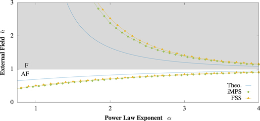
Figure 2. Phase boundary. Critical behavior of the long-range quantum Ising model in the ferromagnetic and antiferromagnetic case as a function of the power law exponent α. We compare the theoretical approximation (Theo.) based on a truncated Jordan Wigner transformation, the infinite MPS results (iMPS), and the finite size scaling (FSS) of the MPS results. The boundary between the gray and white shading is the critical point in the limit  corresponding to the nearest-neighbor quantum Ising model. We observe that both cases react differently when increasing the long-range interactions. In the ferromagnetic case the paramagnetic phase decreases at cost of the ferromagnet, while the antiferromagnetic phase becomes smaller in the other case due to the concurrency in the staggered order. All three different methods show these trends, although they show in the regime α significant relative differences above 0.1.
Download figure:
Standard image High-resolution imageDuring the numerical simulations we follow two different paths. First we use the iMPS algorithm [20, 22] to search for a translationally invariant ground state for a unit cell of q sites. We search for this kind of ground state for q = 2, although the Hamiltonian in equation (1) fulfills translational invariance in the thermodynamic limit for any q. The energy is minimized via variational methods and the strong finite size effects at the boundaries due to the long-range interactions are avoided. Second, we consider finite size systems with a number of sites  and approximate the critical point in the thermodynamic limit
  via finite size scaling. On the one hand this is an appropriate check on the results. On the other hand, we use finite size systems for the dynamics later on and provide a prediction for finite size effects commonly present in quantum simulators. To identify the critical point we keep α and J fixed and iterate over the transverse field h. The von Neumann entropy as a function of the external field has a maximum located at the critical value of the external field
  . For the nearest-neighbor model the critical point can be found based that the area law for entanglement is violated for gapless states [49], where the entanglement is measured with the von Neumann entropy. Although long-range models may in general violate this area law away from the critical point, we take the same approach knowing that the ground state obeys the area law for the two limiting cases
  and
and  . The Ising model has a closing gap around the critical point and therefore the von Neumann entropy S can be used as indicator for the quantum critical point

where  are the singular values squared of the Schmidt decomposition of the system and χ is the maximum bond dimension controlling the truncation of the Hilbert space. In the finite size systems, the eigenvalues of the reduced density matrices correspond to
  when splitting into a bipartition. The entropy and the entanglement have a unique extremum at the phase transition which must coincident with the closing gap and can therefore be used to identify the critical point. An alternative approach would be to use the correlation length of the system or the maximal gradient in the magnetization, both with respect to the external field. We explore the critical behavior of the infinite chain (triangles) and the finite size scaling results (diamonds) in figure 2.
In conclusion, the relative difference between the iMPS and the theoretical estimate is bound by 0.37 (0.17) for the ferromagnetic (antiferromagnetic) model considering  . The relative difference for two arbitrary values x and
  is defined as
  . The actual trend with the difference between iMPS and the theory curve vanishing in the limit
  reflects the analysis in section 3. Further we state that the relative difference between iMPS and finite size scaling results are below 0.11 (0.04). The details on the finite size scaling are described in appendix
5. Scaling of defect density for the Kibble–Zurek hypothesis under a quantum quench
We now turn our focus to the dynamics of the LRQI model. We analyze the quench through the quantum critical point by means of finite systems. We first analyze measurable observables during the quench and then determine the Kibble–Zurek scaling according to the final state, that is a power-law describing the generation of defects as a function of the quench time and a critical exponent. The linear quench for a time dependent external field is defined as

and replaces the coupling h in equation (1). τ is the total time of the quench. We quench from  to
to  . When considering our observables during the quench, we stay close to experimentally realizable measurements. In figure 1 we presented the average magnetization

This is e.g. measurable in cold ion experiments [4]. We choose to plot the magnetization in the x-direction which is measurable in the ferromagnetic and antiferromagnetic case, and can not average out in the simulations due to superpositions, e.g. the ferromagnetic ground state  , and h = 0:
  has no net magnetization for a local measurement of
  . We note in figure 1 for
  the steep gradient around
  , which corresponds to the critical value for the transverse field in the ferromagnetic case treated here. Therefore, we extract the first maximum of the gradient disregarding all minor fluctuations and plot them over α in figure 3. We see a similarity to the critical value of the transverse field from the static calculations for big τ, while for faster quenches the deviation from the static result increases. We present the analogous analysis for the antiferromagnetic case as well in figure 3. For faster quenches the maximal gradient is again below the static result leading to the assumption that this effect is due to a delay during which the system takes time to react. The antiferromagnetic case shows an additional effect as a function of α: longer-range interactions exhibit an extra delay in their maximum gradient. If we consider the antiferromagnetic quench for
  in figure 3(a), the maximum of the gradient moves from
  for
for  to values of
  for
for  . One suggestion to explain this is the concurrent spin configuration in the staggered order in the antiferromagnet which grows for smaller α and might cause this extra delay to establish an antiferromagnetic state. The results on this analysis vary if the quench scheme is not symmetric around the critical point
  .
.

Figure 3. Dynamics and phase boundaries. Around the critical value of the transverse field  , the gradient of the magnetization in the x-direction has its maximum. The system needs time to react to the change and therefore fast quenches with a low quench time τ reach the maximum in the gradient at later times. (a) The first maximum during the quench for the antiferromagnetic model. Instead of the time we show the corresponding transverse field h(t) divided through the corresponding critical field. The small plateaus arise from the discretized measurements. (Remark: small maxima (0.5 times max gradient) in the gradient are neglected.) (b) Analogous to (a) for the ferromagnetic case (same legend as (a)). The analysis failed for the data point with
  and
and  , which was filled with the unconnected point from the simulation with
  . (Jump for fast quenches and small α appears for both bond dimensions.)
Download figure:
Standard image High-resolution imageNext, we present results for a non-global spin measurement. Such a measurement of a single spin in an optical lattice is technically possible [50] and can be realized in cold ion experiments, too. In figure 4 we show the nearest-neighbor spin–spin correlation in the z-direction for the antiferromagnetic case as a function of time and site in the system. As mentioned above, local measurements of  average out due to symmetry apart from numerical fluctuations. Correlations grow during the quench, and finite system boundary effects are visible at both ends of the chain. The total quench time is
  , the system size L = 128, and
  in this example, corresponding to dipole–dipole interactions.
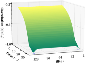
Figure 4. Nearest-neighbor correlation in dynamics. Space–time evolution of the z spin–spin correlation during the quench into the antiferromagnetic phase where the correlation between sites i and  builds up as the external field vanishes. As expected for staggered order in an antiferromagnetic state the correlation is negative. Further we point out more strongly negative correlation due to boundary effects at the end of the quench, where the affected region is indicated with arrows (
 ).
).
Download figure:
Standard image High-resolution imageNow we turn to the Kibble–Zurek hypothesis in the quenches already discussed above. The KZM [26, 41, 51] predicts a scaling of the defects in the quantum system as a function of the quench time τ. We recall that the scaling for the nearest-neighbor Ising model is [52]:

where we use ρ for the defect density, and ν and z for the critical exponents. We have already considered a one-dimensional system in equation (22). Furthermore, equation (22) and the following analysis applies only to linear quenches defined over  , but extensions for the Kibble–Zurek scaling to nonlinear quenches are possible [53]. Plugging in the critical exponents for the nearest-neighbor QI model with
  and z = 1 we obtain
  . The exponent 1/2 is a checkpoint for the calculations in the nearest-neighbor limit
  . The match between theory and experiment does depend on the experimental realization, but yields all over a power law for the defects according to the review in [41].
We are interested in how much the exponent changes when tuning α for the long-range interactions and how it deviates from the 1/2 in the nearest-neighbor case. We estimate the exponent μ in the proceeding analysis which is defined as

Although the scaling can be used in more general cases, we restrict ourselves to the linear quenches crossing the quantum phase transition located at the critical value  analyzed in the previous section 4. This quench scheme starting at twice the critical value was discussed in equation (20). The quench starts in the paramagnetic phase and ends in the ferromagnetic/antiferromagnetic phase. When we are considering the ferromagnetic ground state, the number of defects corresponds to the number of kinks, respectively domain walls, and we use the defect density ρ defined as the number of kinks per unit length and introduced in detail in appendix
  , where the measure is best defined, as the defects are clearly identifiable in terms of the kinks. The data in figure 5, is obtained from simulations based on systems with L = 128 and evolution with the TDVP [21] at
  . We expect that the critical exponent μ approaches 0.5 in the limits
  and
and  resulting in the ferromagnetic nearest-neighbor QI model in the thermodynamic limit. We provide a brief overview of the finite size effects in nearest-neighbor model in appendix

Figure 5. Kibble–Zurek scaling for the long-range quantum Ising model. The exponent μ relates the quench time to the defect density ρ for the power law exponent α as in equation (23). The ferromagnetic model has smaller μ's for longer-range interactions. The defect density grows slower for longer-range interactions for faster quenches regardless of their original density. Two outliers in the data with large errors bars ( and 3.8) have failed to converge and are replaced with simulations with lower bond dimension showing that there is no singularity. In contrast, for the antiferromagnetic model μ stays constant within the error bars and the defects increase at the same rate independent of long-range interactions, but do not necessarily have the same number of defects at the beginning. One non-converging point is not displayed (
 ). The error bars for both cases show the standard deviation from the fit of the critical exponent for the different quench times and do not contain truncation errors of the time evolution.
Download figure:
Standard image High-resolution imageHowever, these results just discussed for the ferromagnetic case are not true for the antiferromagnetic model. The critical exponent stays constant independent of the long-range interaction. The deviation from the nearest-neighbor case  should be due to finite size effects. But we know from figure A4 that the density of defects is again higher for longer range interactions. The defect density of the antiferromagnetic model is defined analogously to the ferromagnetic model: a missing kink in the staggered order is one defect.
6. Conclusion and open questions
In this study we have established that the introduction of long-range interactions changes the physics of one-dimensional quantum spin systems non-trivially as observed in various aspects of the statics and the defect density and therefore merits further attention. This is not limited to the QI model, e.g. the Bose–Hubbard and many other models could be discussed under the influence of the long-range interactions such as dipole–dipole interactions. First we summarize the results from our study of the LRQI model and then raise open problems associated with long-range quantum physics.
We have presented multiple aspects of LRQI model, e.g. the Kibble–Zurek scaling, which lead to a better understanding of physical systems with long-range interactions, e.g. the scaling of generated defects during the quench through a quantum critical point. For the ferromagnetic case we find a slower increasing defect density in comparison to the nearest-neighbor limit when increasing the quench velocity. The defect density is higher in comparison to the nearest-neighbor model for the same quench time. Our simulations give a detailed picture of the critical value of the transverse field in the thermodynamic limit using iMPSs along with a practical guidance how to resolve issues introduced by degeneracy in those systems. We also presented an alternative to the infinite size algorithm using finite size scaling methods to obtain the value of the critical external field in the thermodynamic limit. This uncovers the finite-size effects, which will certainly be present in experiments with small system sizes. The relative difference for the value of the critical point between L = 32 and L = 512 is approximately 15% for the antiferromagnetic case for  . The same comparison for the ferromagnetic yields a relative difference of around
  . The iMPS and finite size scaling phase boundaries are supported by an approximate analytical result using a truncated Jordan–Wigner transformation approach in combination with the Kitaev model. We introduced the dynamics of the LRQI model through local and global observables during a quench from the paramagnetic phase into the ferromagnetic and antiferromagnetic phases crossing the critical point. We related those measurements to the actual quantum critical point through the maximum of the gradient of average global magnetization in the x-direction and analyzed how this is affected by the total time of the quench. Finally, we evaluated the scaling of defects in the Kibble–Zurek scenario leading to the result of a slowly increasing (constant) defect density at the end for increasing quench velocity in comparison to the nearest-neighbor limit of the ferromagnetic (antiferromagnetic) LRQI model. This is reflected in the exponent of the Kibble–Zurek scaling, e.g. in the ferromagnetic case we observe exponents in the range from
  to
to  for power law exponents
  , where
  is the limit of the nearest-neighbor QI model in the thermodynamic limit.
Having concluded our study, we point out open problems that can be addressed in future research. As indicated by the list of the recent studies concerning the dynamics of the LRQI model [18, 34, 36, 37], static physics has been well explored [30–32], but near-equilibrium dynamics such as the Kibble–Zurek hypothesis remain largely unknown, let alone far-from-equilibrium dynamics. One aspect which could be explored in statics and dynamics is the extension to two or higher dimensional systems which we have excluded due to the limitation of MPS algorithms to one spatial dimension for studies of this kind. Two-dimensional setups allow more options for quantum computation to apply gates [48]. In the case of the antiferromagnetic case triangular lattices can lead to the similar concurrence of the staggered order than for long-range interactions in the one-dimensional case. While two-dimensional systems might be accessible through simulations with tensor network methods such as projected entangled pair states (PEPS) [25], this route seems to be more accessible for experiments for any of the models mentioned before. Discrete truncated Wigner methods are another tool to approach two-dimensional systems with numerical simulations [54]. A further path starting from here is the investigation of dynamical phase diagrams. Where recent studies treat e.g. binary pulses in regards to interaction and transverse field of the QI model [55], further possibilities considering time-dependent periodic long-range interactions arise. One study obtaining a dynamical phase diagram for the LRQI chain in the infinite limit using iMPS is [56]. So called completely interacting models at  form another topic for research.
We have shown that the LRQI model is a good starting point for any kind of long-range study. Other models may show new behaviors when including long-range interactions. We think here of the generalization of the QI in terms of the XY-model with a realization in Rydberg systems [57] or the XYZ-model as realized in polyatomic molecules [58]. Furthermore, this includes Hubbard models such as the Bose–Hubbard model, Fermi–Hubbard model as they appear e.g. for molecules. For macroscopic quantum tunneling in the Bose–Hubbard model [59] results might change if the distance of the long-range interaction is larger than the width of the barrier. Other problems suitable for extension to long-range interactions include the quantum rotor model and the bilinear biquadratic spin-one Hamiltonian [60].
Acknowledgments
We acknowledge useful discussions with Jad C Halimeh, Gavriil Shchedrin, and David L Vargas. This work has been supported by the National Science Foundation under grant numbers PHY-120881 and PHY-1520915 and the AFOSR grant FA9550-14-1-0287. The calculations were carried out using the high performance computing resources provided by the Golden Energy Computing Organization at the Colorado School of Mines.
Appendix A.: Numerical methods for long-range statics and dynamics
In this section we describe the numerical algorithms used, which can be skipped by readers not interested in the computational aspects of this work. The motivation for using tensor network methods for the simulation of our systems is their versatile applications for finite and infinite size statics and finite systems dynamics. Since the invention of the finite size version of MPS [61], various tensor network methods have been proposed. These types of tensor networks include for pure states tree tensor networks [62], multiscale entanglement renormalization ansatz [63], and PEPS [64]. All approaches are based on a parameterization of states in the Hilbert space in order to capture many-body physics which is well beyond the reach of exact diagonalization. For an overview we refer to [19]. We divide our description of the specific methods used into three parts. First, we discuss the convergence of the iMPS algorithm used to determine the phase boundary in terms of the critical external field  as a function of the interaction decay α. This algorithm is based on variational methods to find the ground state of a translationally invariant unit cell. Second, we treat the path to finite size simulations via MPS returning the ground state of a system of size L. Iterating over different system sizes L, we discuss how to obtain the critical value of the external field
  in the limit
  via finite size scaling. Third, we complete the section with a discussion of the dynamic results obtained with the TDVP [21] which is able to intrinsically capture long-range interactions and is therefore preferable over a Suzuki–Trotter decomposition as used in many implementations of MPS/TEBD libraries.
A.1. Static simulations: infinite systems and the finite size scaling approach
We explain the numerical methods behind the simulation data shown in figure 2. The iMPS algorithm is designed to find the ground state of an infinite system without boundary effects, returning the translationally invariant unit cell of size L. New sites are inserted in the middle of the existing system and variationally optimized in order to converge to the ground state. The previous iteration is included as the environment, where environment is understood in the sense that it exchanges quantum numbers with the system, and not in an system-bath open quantum system context. In the first step of the algorithm, the unit cell is optimized without any environment; in the second step the solution of the first step is considered as the environment. From that point on the environment grows subsequently with each step. The algorithm terminates if the newly introduced sites fulfill the orthogonality fidelity condition:

where n indicates the iteration step and R is the right part of the system excluding the site introduces in the most recent step. Therefore, the density matrices  and
and  represent the same part of the system and the latter one has one more update included. When the overlap is sufficiently big, the update did not change the result any more. We refer to [20, 22] for a detailed description. The phase boundary for the infinite MPS simulation is obtained for each value of α evaluating the maximum of the bond entropy iterating over the external field h. The bond entropy is defined by the von Neumann entropy introduced in equation (19). We obtain the singular values squared λ when splitting the unit cell of the infinite MPS into the bipartition. The bond entropy is one of a variety of possible entanglement measures [65, 66], and it is based on the Schmidt decomposition separating a quantum system into bipartitions. The entanglement can be measured via the number of singular values, the Schmidt number, or the entropy of the singular values according to equation (19). For example, a Bell state has Schmidt number 2 and von Neumann entropy
  , while an unentangled product state has Schmidt number 1 with von Neumann entropy 0. The maximum of the bond entropy is found using a grid of 21 points ranging from
 ![${h}_{\min }^{[1]}=0.9$](https://content.cld.iop.org/journals/1367-2630/19/3/033032/revision2/njpaa65bcieqn109.gif) (
(![${h}_{\min }^{[1]}=0.0$](https://content.cld.iop.org/journals/1367-2630/19/3/033032/revision2/njpaa65bcieqn110.gif) ) to
) to ![${h}_{\max }^{[1]}=3.9$](https://content.cld.iop.org/journals/1367-2630/19/3/033032/revision2/njpaa65bcieqn111.gif) (
(![${h}_{\max }^{[1]}=2.0$](https://content.cld.iop.org/journals/1367-2630/19/3/033032/revision2/njpaa65bcieqn112.gif) ) in the ferromagnetic (antiferromagnetic) long-range Ising model. We run this evaluation for 51 different values of α ranging from
) in the ferromagnetic (antiferromagnetic) long-range Ising model. We run this evaluation for 51 different values of α ranging from  to
to  . The critical value
 ![${h}_{\mathrm{crit}}^{[1]}$](https://content.cld.iop.org/journals/1367-2630/19/3/033032/revision2/njpaa65bcieqn115.gif) is the grid point with the maximal bond entropy. Based on this result, we refine the search on the next grid defined as
is the grid point with the maximal bond entropy. Based on this result, we refine the search on the next grid defined as

where ![${{dh}}^{[i-1]}$](https://content.cld.iop.org/journals/1367-2630/19/3/033032/revision2/njpaa65bcieqn116.gif) is the step size on the grid. The results presented in section 4 and in the following convergence studies are for
is the step size on the grid. The results presented in section 4 and in the following convergence studies are for ![${h}_{\mathrm{crit}}^{[2]}$](https://content.cld.iop.org/journals/1367-2630/19/3/033032/revision2/njpaa65bcieqn117.gif) , that is the external field at the quantum critical point between the paramagnetic and ferromagnetic, or antiferromagnetic phase. The superscript denotes the iteration refining the grid for the search and has no physical meaning past an indication for the precision of
, that is the external field at the quantum critical point between the paramagnetic and ferromagnetic, or antiferromagnetic phase. The superscript denotes the iteration refining the grid for the search and has no physical meaning past an indication for the precision of  .
.
We now discuss convergence of the iMPS results. We take the default convergence parameters of the OSMPS library [29] with the modification of an iterative bond dimension of  . In figure A2(a) we show the difference in bond entropy
  ,
,  , and
, and  . These results call for a technical discussion of this behavior due to the large difference for many points with
  , here in the antiferromagnetic case. This behavior is related to symmetry breaking. The degenerate ground state in the limit
  is the GHZ state

but without enforcing  any superposition of
  and
and  minimizes the energy of the system. Therefore, the bond entropy can be between the bond entropy S = 0 of a product state and
  of the GHZ ground state. We discuss the origins of this problem related to the numerical algorithm of iMPS. Tracking the singular values, we find either a distribution of pairs in the states with high entropy corresponding to the two different signs as pointed out in the limit
  for the GHZ state in equation (A.3). The low entropy states have decaying non-degenerate singular values. The iMPS algorithm selects one of the degenerate states at non-predictable points due to the randomized initial state at the very beginning of the algorithm, as well as the entanglement truncation step, which can randomly pick a particular parity sector for the environment. This is related to the dominant eigenvector of the transfer matrix (see [20]). Note that, once one of the broken symmetry states
  or
or  becomes more dominant, this dominance is 'stored' for all subsequent iterations in the environment in the iMPS algorithm. Hence, symmetry breaking by random random numerical noise cannot be removed by running more iterations. The higher bond dimension and the number of iterations in the algorithm lead to smaller differences in the pairs of degenerate singular values until one of the dominant eigenvectors of the transfer matrix is kept and the other truncated. For
  , the difference in the leading singular values is
  decreasing to
  for
for  . Therefore, the singular values double in magnitude since an equal counterpart was neglected. In summary we can state the following: (1) For
  symmetry breaking is not resolved. The result converges, as expected, better for faster decaying long-range interaction up to 10−3 between the results for
  and
and  . (2) For
  we truncate one of the symmetry broken states for
  meaning that the difference in entropy is large for any comparison to
  . The results with bond dimension 20 have an error between 10−1 and 10−2 with regard to
  . The singular values for
  are close enough to be resolved as degeneracy leading to the conclusion that the state is also well converged. (3) The region in between the algorithm alternates between resolving the symmetry broken ground state or not, leading to convergence up to 10−4. The same trend can be stated in the ferromagnetic case shown in figure A2(b). A corresponding example for the degeneracy evolving in the singular values can be seen in figure A1. We emphasize that this analysis is relevant if searching for the maximal entropy on a very coarse grid or when trying to show convergence across bond dimensions. For a single bond dimension we may use the final value of the orthogonality fidelity described in equation (A.1). The convergence in terms of the orthogonality fidelity is discussed in appendix C.
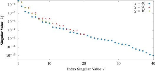
Figure A1. Degenerate singular values in iMPS. The key for understanding the convergence of the bond entropy is Λ, the singular values squared, shown for different bond dimensions χ. The difference in entropy is here related to the symmetry breaking appearing for  . In contrast the singular values for
  and
and  appear in pairs. Considering the convergence with regards to χ by means of the bond entropy fails for this reason. This example represents a simulation for
  and h = 1.14 in the ferromagnetic model.
Download figure:
Standard image High-resolution image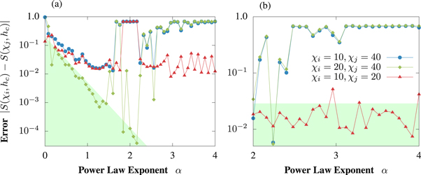
Figure A2. Convergence of iMPS. (a) In the antiferromagnetic model on the left part of the plot we see the expected behavior that the error is increasing for longer-range interactions. This is indicated by the shaded green triangle, where values within the triangle have broken the symmetry or not for both bond dimensions  and
and  . In contrast on the right part of the plot we have one simulation with conserved symmetry and one with broken symmetry for the comparison between
  and
and  . (b) In the range shown in the plot for the ferromagnetic case, the degeneracy is never kept up to
  so that the error
  is not a reasonable basis on which to judge convergence. But the simulations comparing
  and
and  in the shaded green rectangle are a meaningful error with regards to the iMPS symmetry breaking issue. Legend applies to both (a) and (b).
Download figure:
Standard image High-resolution imageThe finite size simulations have a two-fold purpose. On the one hand, finite size scaling provides an alternate route to obtain the thermodynamic limit of the system and is therefore a check against the iMPS results. While iMPS simulations are only limited by the bond dimension used, finite size simulations enforce the  symmetry and avoid for this reason the symmetry-breaking effects discussed in the previous section. On the other hand, we see the finite size effects affect the system, which is important as the dynamic simulations are for finite systems. For the finite size scaling we use the same grid method as for iMPS before with the initial grid boundaries
 ![${h}_{\min }^{[1]}=0.8$](https://content.cld.iop.org/journals/1367-2630/19/3/033032/revision2/njpaa65bcieqn157.gif) (
(![${h}_{\min }^{[1]}=0.0$](https://content.cld.iop.org/journals/1367-2630/19/3/033032/revision2/njpaa65bcieqn158.gif) ) and
) and ![${h}_{\max }^{[1]}=9.8$](https://content.cld.iop.org/journals/1367-2630/19/3/033032/revision2/njpaa65bcieqn159.gif) (
(![${h}_{\max }^{[1]}=2.0$](https://content.cld.iop.org/journals/1367-2630/19/3/033032/revision2/njpaa65bcieqn160.gif) ) with nine (seven) grid points for each α and L in the ferromagnetic (antiferromagnetic) case. We refine the grid four times after the initial run ending with the bond dimensions
) with nine (seven) grid points for each α and L in the ferromagnetic (antiferromagnetic) case. We refine the grid four times after the initial run ending with the bond dimensions  for the iteration over the OSMPS convergence parameters. The final distance between points is for both cases
 ![${{dh}}^{[5]}\approx 0.004$](https://content.cld.iop.org/journals/1367-2630/19/3/033032/revision2/njpaa65bcieqn162.gif) . For the refinement we find
. For the refinement we find ![${h}_{\mathrm{crit}}^{[i]}(\alpha ,L)$](https://content.cld.iop.org/journals/1367-2630/19/3/033032/revision2/njpaa65bcieqn163.gif) with the bond entropy at the middle of the system and construct the next, refined, grid
with the bond entropy at the middle of the system and construct the next, refined, grid  in the interval
 ![${h}_{\mathrm{crit}}^{[i]}(\alpha ,L)\pm {{dh}}^{[i]}$](https://content.cld.iop.org/journals/1367-2630/19/3/033032/revision2/njpaa65bcieqn165.gif) . The maximum number of sweeps are
. The maximum number of sweeps are  for the corresponding iterations in bond dimension
  . The other convergence parameters, which stay constant for each set of convergence parameters iterated over, are a variance tolerance of 10−10 and a local tolerance of 10−10. For power law exponents of
  , we actually reach a variance superior to 10−7 where simulations converge better away from the critical value for the ferromagnetic Hamiltonian. In the antiferromagnetic case, longer-range interactions show worse convergence independent of the critical value of the external field. We discuss the details in appendix B. The critical values are evaluated for system sizes 32, 64, 128, 256, and 512. By using finite size scaling, we obtain the critical value
  of an infinite system. From Cardy [67] we know that for a finite system the distance of the critical point
  to the critical point in the thermodynamic limit
  can be described by

Knowing that the values of  are increasing in the ferromagnetic and antiferromagnetic case according to figure A3, we can use

and fit the unknown parameters  , ν, and c via [68]. Due to the logarithmic choice of the system size, small system sizes are overrepresented in the fit. We account for this by assigning an uncertainty proportional to
  at each data point. The results for different system sizes and the data from the finite size scaling can be seen in figure A3. In the antiferromagnetic case (a), the points show the expected behavior with smaller spacing between bigger system sizes; thus the simulations are converging to the thermodynamic limit. When the interactions are not decaying for
  , the finite size scaling breaks down due to poorly converging simulations. The black curve represents the
  limit achieved through the finite size scaling fit. Figure A3(b) shows the same behavior for the ferromagnetic case. We point out that the weights for each data point are necessary in this case to avoid an intersection of the curve for
  with the finite size solution L = 512 for longer-range interactions.
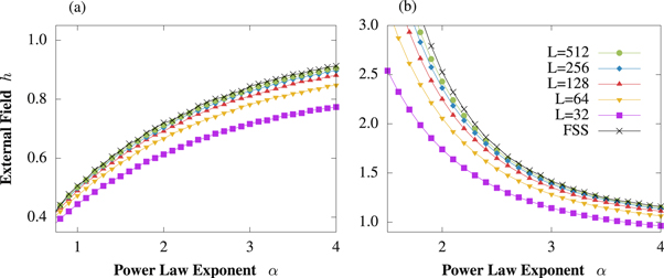
Figure A3. Finite size scaling for the long-range quantum Ising model. Finite-size effects lead to a decrease of the critical value of the external field  for smaller system sizes. Furthermore we achieve the thermodynamic limit for infinite system size via finite size scaling (FSS). (a) Antiferromagnetic case; (b) ferromagnetic case. Legend applies to (a) and (b) both. We point out that for the limit
  and
and  the ground state for the ferromagnetic case is always the GHZ state, while the antiferromagnetic case has an exponential degeneracy. The latter might contribute to convergence problems when α is approaching zero. The limits
  is equal to the nearest-neighbor case and all limits
  have a ground state aligned with the external field.
Download figure:
Standard image High-resolution imageA.2. Dynamic simulations with MPS
In this section we analyze the scaling of the numerical simulation with regards to the Kibble–Zurek hypothesis. The KZM describes the scaling of the defect density when driving a quantum system through a quantum phase transition and was originally formulated in terms of cosmology [69], and later brought to quantum systems such as helium [70] or the nearest-neighbor QI model [26]. There, the external field is changed in order to cross the quantum critical point at  in the nearest-neighbor QI model. In our analysis the quantum critical point
  depends on the actual value of the power law exponent α as presented in section 2.
In order to analyze the Kibble–Zurek hypothesis in the present of long-range interactions, we first define the defect density for the ferromagnetic model. The defect density was defined in [71] using nearest-neighbor correlations, and we divide by  instead of L to account for the open boundary condition:

We now shortly outline why this works in the ferromagnetic case for the nearest-neighbor model. We recall that at the end of the quench the external field h = 0 and therefore the ground states  are defined through

This is equivalent to the GHZ state and we recall that this is the ground state before  symmetry breaking. The first excited state has
  degeneracies and is described by a single kink in the system, e.g.
  . The number of kinks is equal to the number of excitations. If we consider first a state with a product state of only spins up or down, one is easily convinced that equation (A.6) describes the defect density. For every domain wall the nearest-neighbor correlation inside the sum contributes, while for spin inside the domain wall the term is canceled. Moreover, it is a reasonable measurement even when the spins are changing slowly. Let us verify this point with an example of three spins changing from up to down,
  . The subscript reflects the basis if it differs from z. The measurement of the correlation yields zero in both cases:

The measurement in equation (A.6) yields one defect, as expected, with the spins flipping once over the chain. We emphasize that this cannot be used in any region with  , except as an approximation for
  . Let us turn to the defects of the ferromagnetic LRQI model. The defects are local kinks, but the states with one kink are not all degenerate. In fact, the energy gap to the ground state is smaller for kinks closer to the boundaries. This is a manifestation of the boundary effects. Counting all kinks equally, we make an error growing in the limit
  . The defect density of the antiferromagnetic case in the nearest-neighbor model is defined as

We again point out that the single defects have a different excitation energy depending on their position in the bulk.
In order to retrieve the critical exponent scaling in the form of equation (23), we simulate the quenches for L = 128 for the set of τ's containing  . For each α we fit the coefficient c and the critical exponent μ via [68]. In order to estimate if any non-converged simulations are included in the data, the standard deviation
  is calculated through the covariance matrix given by the fitting function. In figure A4 we show one example in the ferromagnetic model for
  and 4. The error of the fit can be seen as an indicator for the validity of the dynamic results. Running simulations with different χ helps us to identify failing simulations versus singularities. For weaker long-range interactions with big α the fits reproduce the results while for longer-range interaction the procedure fails (
 ). The initial state is based on the same convergence parameters as the statics discussed in appendix A.1, except for the bond dimension which is lowered to
  or 100. For the dynamics we keep the corresponding maximal bond dimension and use the default TDVP convergence parameters in OSMPS [29] for all other parameters.

Figure A4. Fitting the exponent for the defect density in the Kibble–Zurek hypothesis. (a) Examples for the defect density at the end of the quench for the antiferromagnetic long-range quantum Ising model plotted over the quench time τ for different power law exponents α shows the decrease in defect density for slower quenches. The power law in the scaling leads ideally to a line in the log–log plot which is here slightly affected by failing simulations. This is especially evident for small α, e.g. in the antiferromagnetic case for  and
and  . (b) Corresponding data for the ferromagnetic model.
Download figure:
Standard image High-resolution imageAppendix B.: Convergence of finite-size statics
In the appendix we briefly address the convergence of the finite size statics. We already discussed the convergence of iMPS in appendix A and therefore it is known that the convergence can be studied in different fashions. In OSMPS, the variance of H is considered for statics of finite size systems. The user chooses a value, we take 10−10, and OSMPS iterates through the different bond dimension χ. We consider  and
and  of the last grid. This fifth grid has a discretization of
  (ferro) and
  (antiferro) around the critical point of the fourth grid. The output contains the flag if the simulation converged according to the value for each χ; in addition the actual value of the variance is saved as well.
We start to look if the simulation converged with a variance of  . This information is contained in the left part of figure B1 for the ferromagnetic model. The coloring is as follows: green for convergence at the first convergence parameter with
  , red for convergence the second convergence parameter at
  , and blue if not converged at either of the previous bond dimensions. In order to estimate the variance of the blue region, we plot the actual value for the critical value
  as a function of α and system size in the right part of figure B1. For the analysis used in the main part of the paper we achieve a variance less than 10−7.
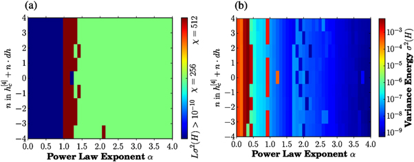
Figure B1. Convergence of finite size MPS ground states: built-in convergence check of OSMPS using the variance of H for the last grid and L = 512 in the ferromagnetic case. (a) The critical region causes most problems to converge up to variance  (green converged with
  , red converged with
  , blue not converged). (b) The actual variance of H of the fifth grid for the results used in the main section is at least converged around 10−6.
Download figure:
Standard image High-resolution imageWe follow the similar scheme to study the convergence in the antiferromagnetic LRQI Hamiltonian, presented in figure B2. The convergence becomes in general more difficult in the longer-range interacting region with  , still reaching a variance of 10−6 or better for the shorter-range region with
  .
.

Figure B2. Convergence of finite size MPS ground states: built-in convergence check of OSMPS using the variance of H for the coarse grid and L = 512 in the antiferromagnetic case. (a) The longer-range interaction region causes most problems to converge up to variance  (green converged with
  , red converged with
  , blue not converged). (b) The actual variance of H of the fifth grid is shown on the right. Some antiferromagnetic simulations did not finish in the allotted time.
Download figure:
Standard image High-resolution imageAppendix C.: Convergence of infinite-size statics
We discussed at length that it is difficult to study convergence as a function of the bond dimension in terms of the bond entropy in appendix A.1. But we give in the following a brief overview of the convergence of the iMPS in terms of the orthogonality fidelity defined in equation (A.1). In order to show convergence it is convenient to switch from the orthogonality fidelity to the actual error, the infidelity

Figure C1 shows the convergence for the antiferromagnetic and the ferromagnetic model for the highest bond dimension  of our convergence parameters and the second grid. In terms of the orthogonality fidelity the simulations are well converged at an error
  of 10−8 or better for
  . Convergence close to the critical point is in general worse. For
  interaction become too long-range to converge at the same level for these convergence settings. We remind the reader that the search interval for the ferromagnetic case shown in figure C1(b) does not contain the critical value for very small α with an upper bound of
  .
.

Figure C1. Convergence of the iMPS. We consider the infidelity of the orthogonality fidelity plotted as logarithm of base 10. Both the ferromagnetic case (a) and the antiferromagnetic case (b) convergence for  mostly to an infidelity of 10−8 or better. Non-converging points are typically around the critical point of the model moving downwards for the antiferromagnetic case and upwards for the ferromagnetic case. The vertical stripes originate in the fact that each simulation might have a different critical value from the first grid, where
  is identical within one strip.
Download figure:
Standard image High-resolution image
Appendix D.: Finite size effects in the Kibble–Zurek scaling
Section A.2 raised the question of how finite size effects influence the value of the critical exponent μ in the dynamics. We consider the quench times  and different system sizes
  to show these finite size effects in the nearest-neighbor limit. This limit corresponds to
  . Table D1 presents the data. The error is solely from the fit and does not contain truncation error or methological errors from the time evolution. The thermodynamic limit is obtained via finite size scaling using the following approach:

The value  is shown in the last column of table D1. As in the finite size scalings previous discussed, we weight the data points for large system sizes more since we have less data points in the corresponding interval. We do not show the error here, because of the limited number of data points with regards to the degrees of freedom. In conclusion, the data supports the assumption that the finite size effects are relevant and the thermodynamic limit in the nearest-neighbor model approaches
  in both the ferromagnetic and antiferromagnetic case.
Table D1. Finite size effects in the Kibble–Zurek scaling for the quantum Ising model. The finite size effects lead to a growing critical exponent for smaller system sizes. In the thermodynamic limit the critical exponent of 0.5 is reached.
| System size | L = 32 | L = 64 | L = 128 | L = 256 |

|
|---|---|---|---|---|---|
| Anitferro | 0.810 ± 0.060 | 0.614 ± 0.026 | 0.532 ± 0.016 | 0.502 ± 0.017 | 0.48 |
| Ferro | 0.810 ± 0.060 | 0.614 ± 0.026 | 0.532 ± 0.016 | 0.500 ± 0.017 | 0.48 |