


Abstract
Crystal dislocations govern the plastic mechanical properties of materials but also affect the electrical and optical properties. However, a fundamental and quantitative quantum field theory of a dislocation has remained undiscovered for decades. Here we present an exactly-solvable one-dimensional quantum field theory of a dislocation, for both edge and screw dislocations in an isotropic medium, by introducing a new quasiparticle which we have called the 'dislon'. The electron-dislocation relaxation time can then be studied directly from the electron self-energy calculation, which is reducible to classical results. In addition, we predict that the electron energy will experience an oscillation pattern near a dislocation. Compared with the electron density's Friedel oscillation, such an oscillation is intrinsically different since it exists even with only single electron is present. With our approach, the effect of dislocations on materials' non-mechanical properties can be studied at a full quantum field theoretical level.
Export citation and abstract BibTeX RIS
Changes were made to this article on 1 February 2017. The acknowledgments were updated.
1. Introduction
Crystal dislocations are a basic type of one-dimensional topological defects in crystalline materials [1]. Since Volterra's ingenious prototype in 1907 [2], and Taylor, Orowan and Polyani's simultaneous formal introduction in 1934 [3–5], a dislocation has been shown to have strong influences on material properties, including the governing role in the plastic mechanical process, and the widespread impact on the thermal, electrical and optical properties [1, 6]. Since a dislocation can strongly scatter an electron and thereby changes material electrical properties, such as reduces the electron mobility or increases the electrical resistivity, it is of central importance to obtain a theory describing the electron-dislocation interaction, to understand the role of a dislocation in the electronic properties of materials.
In general, the theoretical approaches of studying electron-dislocation interactions can be divided into the following mainstream categories:
- (1)Classical scattering theory: dislocation can be modeled by its partial feature (e.g. dislocation modeled as charged line in certain semiconductors) [7–10]. This allows one to study the electron-dislocation scattering using classical theory, but such modeling has a pure electrostatic origin and does not capture the scattering processes that occur with a genuine dislocation, which contains both strain scattering effects and vibration scattering effects [1, 6].
- (2)Geometrical approach: dislocated crystal is treated as a manifold in a curved space (e.g. spacetime in general relativity) [11–15]. This approach can describe the single electron motion quite well near a dislocation under the framework of the one-particle Schrödinger equation, yet it also experiences some problems such as the cumbersome mathematics caused by a curved metric, limiting this approach to the first-quantized single particle level without a generalization to many-body cases.
- (3)First-principles density functional theoretical calculations: in principle the electronic structure near a dislocation core can be studied. However, due to the long-range nature of a dislocation, it requires one to build a supercell leading to an exceedingly high computational cost. To the best of our knowledge, only ground-state properties such as the atomic configuration near a dislocation core can be studied using this approach [16, 17].
- (4)The classical affine gauge theory of dislocations [18–20]: structurally similar to quantized gauge theory, but is limited only to a classical elasticity field, without being quantized at the time of this study. Since the step of quantization is necessary in order to study the electronic properties properly, the investigation of electronic properties using this approach have not started yet.
However, despite the wide variety of approaches to study electron-dislocation interaction, a unified electron-dislocation interacting theory at a quantum many-body level is still not available. Such a theory is essential to go beyond single-electron picture by taking into account the electron exchange and correlation, and other many-body effects, and is also essential to properly considering the higher-order multiple scattering events. If fact, unlike the case of the electron-point defect interaction where the complete impurity interacting field theory is well established [21], the lack of a field theory of dislocations not only impedes a further understanding of dislocations on material electronic properties at a fundamental many-body level, but also limits the usage of the terms 'impurity' and 'disordered systems' referring to quenched, point defect-related properties under many circumstances [22].
Here, we take a very different approach to study the electronic behavior in a dislocated crystal. Instead of treating a dislocation line as a charged line, or strain field, or a quenched defect, we treat the dislocation itself as a fully quantized object. Based on well-established classical dislocation theory and a canonical quantization procedure, we provide an exact and mathematically manageable quantum field theory of a dislocation line. We find that in an isotropic medium, the exact Hamiltonian for both the edge and screw dislocations can be written as a new type of harmonic-oscillator-like Bosonic excitation along the dislocation line, hence the name 'dislon'. Just as a phonon is a quantized lattice displacement with both kinetic energy and potential energy, a dislon is similar in the sense that it is also a lattice displacement with both kinetic and potential energy, but further satisfies the dislocation's topological constraint  where b is the Burgers vector, L is a closed contour enclosing the dislocation line (denoted as D in figure 1(a)), and u is the lattice displacement vector, i.e. the atomic position deviation occurs after the crystal is dislocated, and du is the differential displacement along the contour L. Using this approach, the scattering between an electron and the 3D displacement field induced by the dislocation can easily be solved via a many-body approach, with the topological constraint
  respected all along this study.
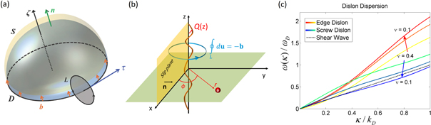
Figure 1. (a) The equivalent definitions of a generic dislocation D, which is denoted as a loop. A dislocation line can be regarded a special case of the dislocation loop. On one hand, a dislocation line D can be defined as  where L is the loop enclosing the dislocation line D. On the other hand, an equivalent definition is based on an arbitrary surface S (blue) with line D as its boundary. A dislocation can be defined as an overall shift of surface S by a constant amount of the Burgers vector b (blue surface is shifted to the yellow one).
  is the coordinate perpendicular to the surface S, and is convenient for defining the strain tensor
  (b) A long dislocation line along z-direction vibrating within slip plane (xz) with
  the transverse displacement. Such vibration shares similarities with a phonon as it is also a quantized lattice displacement, but is constrained by
  where L is an arbitrary loop circling dislocation. An electron located at position r will be scattered by dislocations. (c) Quantized vibrational excitation dispersion relations along dislocation line ('dislon') for both edge (hot-colors) and screw (cool-colors) dislocations at various Poisson ratios ν. The classical shear wave is shown as a linear-dispersive black-dotted line. The classical shear wave is shown as a linear-dispersive black-dotted line, and the arrows indicate a decreasing trend of Poisson ratio for edge (red arrow) and screw (blue arrow) dislons, respectively.
Download figure:
Standard image High-resolution image2. The classical foundation prior to dislocation quantization
To begin with, we provide a self-contained review of the classical dislocation's theory following the logic in [23] and [24]. In spite of the well establishment of the classical dislocation theory, we feel such an introduction necessary since this particular classical theory which facilitates the quantization is not commonly introduced in textbooks or articles in material sciences journals. Defining  as the atomic lattice displacement at spatial point R, the spatial derivative tensor of u, namely the distortion tenstor, can be written as
  from which we define the strain tensor
  as
as

where  are the Cartesian components. The relation between the stress
  tensor and strain tensor
  can be found by the generalized Hooke's law as

where Einstein's summation convention is adopted. In an isotropic medium, the elastic stiffness tensor  (
( is given by

where λ and μ are 1st and 2nd Lamé constants, respectively.
At equilibrium, the internal stress in each direction must balance with the external force  hence the local force equilibrium of the ith component can be written as

Equation (4) is a 2nd order linear inhomogeneous differential equation with respect to the displacement field vector component  which can readily be solved using the Green's function method. Defining the Green's function of equation (4) as

Then the solution of the corresponding inhomogeneous equation (4) can be written from equation (5) as [23, 24]

where i, j, k, l, m = 1, 2, 3 are the Cartesian components. The 2nd equality can be obtained by substituting equation (4) to the 1st equality in equation (6), and using integration by parts. This gives the generic displacement field using the Green's function's approach.
For the convenience of later computation, the Fourier transformed Green's function is also defined as  which can be obtained by taking the Fourier transform of equation (5) as

where  is the Poisson ratio.
The above theory equations (1)–(7) is valid for all types of lattice displacements within the framework of elasticity. For the case of a dislocation as one special type of displacement, we need to introduce a generic and rigorous definition of the dislocation in order to formulate a quantized theory. In realistic materials, dislocation can either form a self-terminated loop, or form a line terminated at crystal surface [6]. In particular, a line can be considered as a special case of an arbitrary loop with the both ends at  joint together [25]. Therefore, we still could picture this generic dislocation as an arbitrary loop, as shown in figure 1(a) and elaborated in [26]. The arbitrary dislocation loop is denoted as the loop D (black circle), with S is an arbitrary surface (blue surface) whose boundary gives this dislocation loop D, and the local tangent vector of the dislocation loop D is denoted by
  The dislocation is defined as a global shift of the whole surface S by an amount of the Burgers vector b (blue surface shifted to the yellow surface nested above, as indicated by the orange arrows). Defining the coordinate
  along the surface normal n (i.e. locally
  is always perpendicular to the surface element
  on the surface S), then we have the distortion
  on the discontinuity surface S, where
  denotes the projection along the surface normal,
  is the component of the discontinuous shift b, and
  comes from the fact that the discontinuity caused by the shift of the surface will be located right at and only at the surface S; hence from equation (1), we have

Substituting equation (8) back into equation (6), and noticing the fact that  since
since  is defined as the direction perpendicular to the local surface element
  the displacement field
  caused by a dislocation loop with Burgers vector
  can finally be re-written as a surface integral over the surface S as

where  is a surface area element on the chosen surface S,
  is a spatial point on the surface S, while R is an arbitrary spatial point which can be well outside the surface S.
To further simplify equation (9), we consider a long, straight dislocation line instead of an arbitrary loop, as shown in figure 1(b) where a long, straight dislocation line extends along the z direction with a core position located at (x0, y0) = (0, 0). This dislocation line would vibrate within a plane called slip plane, which we have defined it as xz plane. Noticing the fact that the discontinuity surface S now evolves into the slip plane xz within which the discontinuity is generated: for an edge dislocation the discontinuity is created along the x-direction, while for a screw dislocation the discontinuity is created along the z-direction. Such vibration has the form of an atomic motion, similar to phonons but they cannot be described as a collection of propagating plane waves. For an edge dislocation, the slip plane is fixed, i.e. an edge dislocation keeps slip within the same plane, while for a screw dislocation, the slip plane is not fixed, i.e. a screw dislocation can slip along different directions at multiple slip steps. However, the dynamic process we are considering in this study is the local vibrational modes before it starts to slip, with a timescale much faster than an actual slip process which requires the shift of an array of atomic positions. Defining  to be the transverse displacement of the dislocation line within the slip plane, along the x-direction at position z, as in figure 1(b), hence the surface area element
  then satisfies
  and equation (9) can be further rewritten as [24, 27]

where  and
and  are 2D and 3D position vectors, bm is the mth component of the Burgers vector and n is the direction perpendicular to the slip plane with the lth component nl. To understand the significance of the dislocation displacement
  we need to bear in mind that
  is not the displacement of the lattice displacement vector
  but a displacement caused by the overall movement of the dislocation line. In fact, the dislocation displacement
  causes the lattice displacement
  in the whole crystal. For a vanishing dislocation displacement
  the lattice displacement still remains finite due to the topological behavior of a dislocation, and a resulted singular behavior which is discussed in detail at the end of this section. Now mode-expanding the dislocation displacement as a Fourier series

where κ is the wavenumber along the z-direction, we can then express the displacement  as [25]

where  is an expansion coefficient to be determined. Substituting equation (11) back into equation (10), and comparing the result with equation (12), we have obtained the coefficients

Now defining the 2D Fourier transformed coefficient  of the expansion coefficient
  as
as
where A is the sample area perpendicular to the dislocation direction, and  is the 2D wavevector. Substituting the 2nd formula in equation (14) back into equation (12), and comparing the result with the Fourier transform of equation (13), we finally obtain

where the 3D wavevector is defined as  Now using equations (12) and (14), the displacement field can then be written in terms of
  as
as

Now we are ready to encapsulate the classical kinetic and potential energies due to the dislocation displacement field. Substituting equation (16) into the expressions for the classical kinetic energy  and potential energy
  the classical Hamiltonian can finally be rewritten in terms of a 1D effective Hamiltonian [27],

where L is the sample length along the dislocation direction,  and
and  are the classical linear mass density and tension, respectively, and can be written down from a classical theory straightforwardly as was done in [27]. For an edge dislocation, we have the effective mass density and the tension written as
while for a screw dislocation, we have
where kD is the Debye cutoff in the in-plane xy direction. Before proceeding to the quantized dislocation theory part, we would like to clarify the implications of the classical dislocation Hamiltonian in equation (17). One might be wondering why a dislocation, which is usually considered as a type of quenched defect without excitation, can be written down through a Hamiltonian form as equation (17). In particular, it appears that for a static, quenched dislocation in the long wavelength limit, there is no displacement with  and the dislocation Hamiltonian equation (17) simply vanishes. However, this is not true since a dislocation is a topological defect which cannot be simply canceled by a local variation of
  This can be seen from equation (15). In the long-wavelength
  limit, the expansion coefficient
  Hence in the static limit, despite the vanishing
  according to equation (11), the divergent expansion coefficient
  will compensate and bring the lattice displacement
  back to a finite magnitude, according to equation (16). In other words, the Hamiltonian equation (17) describes a dislocation as a mathematical entity of the lattice displacement field satisfying its rigorous definition
  regardless of the static quenched dislocation or the dynamic vibrating dislocation. We have to admit that if one insists on taking the static limit, the dislocation Hamiltonian equation (17), instead of simply vanishing, becomes ill-defined, since
  while
while  simultaneously. To separate the contribution from the static electron-dislocation scattering from the dynamic electron-dislocation scattering and determines the sole contribution from the static dislocation, a different approach using the boundary operator method has been implemented [28]. It is also worth mentioning that, contrary to many would naturally expect, a dislocation is more than a quenched defect. For instance in some materials when considering thermal transport, the dynamic scattering can even dominate over the static scattering [29, 30], which have been explained using classical vibration models [27, 31].
3. Canonical quantization of crystal dislocation
After reviewing the classical dislocation theory, we now proceed to the quantization procedure. For a canonical coordinate  we could define its canonical conjugate momentum as
  in which
  is the Lagrangian. Now imposing the following canonical quantization condition between the canonical coordinate
  and conjugate momentum
  that
that

Then the classical dislocation Hamiltonian in equation (17) can be quantized by recognizing  and
and  as first-quantized quantum mechanical operators satisfying equation (20), instead of the classical dynamic variables. The Hamiltonian equation (17) can now be written as

To readily study the effect of a dislocation on the electronic properties at a full many-body level, a second-quantized dislocation Hamiltonian is needed. By defining the creation and annihilation of quantized dislocation modes  and
and  satisfying the canonical commutation relation
 ![$[{a}_{\kappa },{a}_{\kappa ^{\prime} }^{+}]={\delta }_{\kappa ,\kappa ^{\prime} },$](https://content.cld.iop.org/journals/1367-2630/19/1/013033/revision1/njpaa5710ieqn77.gif) equation (20) can further be written as the following equivalent form as
equation (20) can further be written as the following equivalent form as

where  The first-quantized Hamiltonian equation (21) now can be rewrittng using equation (22) as the following Hamiltonian

with eigenfrequencies  Equation (23) has a form as a collection of non-interacting Bosonic excitations. Despite the observation that such an excitation shares the similarity with phonon excitation as a type of quantized lattice vibration, the topological constraint here
  leads to a different excitation quantum along the dislocation line and decay away from the dislocation core, which may suitably be called the 'dislon', to distinguish the dislon from a non-interacting phonon. In particular, by imposing the in-plane Debye cutoff kD, in xy plane for both an edge dislocation (
 and a screw dislocation (
 the dispersion relation
  can be written in a closed form as
where  is the shear velocity, and the four relevant coefficients are

 and
and  The dislon dispersion at various Poisson ratio ν values and constant shear velocity
  are plotted in figure 1(c), where the classical shear wave, or equivalently the transverse acoustic phonon mode
  (black-dotted line) serves as a pre-factor in quantum–mechanical version of dislocation excitation in equation (24). The higher excitation energy of the edge dislon relative to the screw dislon is reasonable, since even in the pure classical picture, the edge dislocation energy density is higher than that of the screw dislocation by a factor of
  [32]. Substituting equation (22) back into equation (16), the displacement field
  caused by a dislocation can finally be written in a second-quantized form as

which is the main result of this section 3 and will be used in section 4.
4. Electron-quantized dislocation interaction
The introduction of the quantized dislocation in section 3 enables us to treat the electron-dislocation scattering at a full second-quantized level by taking advantage the many-body theory as the electron-dislon interaction. We start from a lattice model, where  so that
  is the equilibrium position of an ion with label j, and we assume that there are N atomic sites in the system. Assuming the electron charge density is
  the electron–ion interaction Hamiltonian expanding to the 1st-order approximation can be written as [33, 34]
where the 1st term gives the ion potential function which describes the electrons traveling within the periodic potential of a crystal, i.e. Bloch waves, and the 2nd term describes the scattering by a generic displacement field,

To further simplify equation (27), we note that the electron charge density  can be written in terms of the number density
  as
as

where  is the Fourier-transformed electron number density. In addition, the ionic potential
  can also be expanded in terms of Fourier components by

where q is within 1st Brillouin zone, the Fourier component of a screened Coulomb potential gives  in which
  is defined as the Thomas–Fermi screening wavenumber, and G denotes the reciprocal lattice vectors. Now substituting equations (25) and (29) into the term
  in equation (27), we obtain (supplementary material A)
where we have used the fact that  where N denotes the total number of atoms. Now we further substitute equations (15), (28) and (30) back into the interacting Hamiltonian equation (27), and moreover by assuming a non-Umklapp normal scattering process (G = 0), the electron-dislocation interaction Hamiltonian equation (27) can further be rewritten in a second-quantized form as (supplementary material A)

This equation (31) gives a reasonable prediction. In particular, at  both the dislon excitation equation (24) and electron-dislon interaction equation (31) vanish due to the pre-factor
  This is consistent with the fact that a system with
  corresponds to a purely elastic system without shear modulus (an intuitive example with
  is like rubber), where dislocations simply do not exist.
Now noticing the fact that the creation and annihilation operators  and
and  have only momentum indices κ along the dislocation direction, and using the fact that
  then equation (31) can further be simplified by performing a summation in the 2D
  plane perpendicular to the κ direction (supplementary material B)

Equation (32) is capable of treating the interaction between one dislocation and multiple electrons by modeling the election density  For a single electron located at
  as shown in figure 1(b), we have the Fourier transformed electron density
  and equation (32) can be further simplified as (supplementary material B)

in which the position-dependent electron-dislon coupling coefficient  is defined as

where  is the nth order Bessel function of the 1st kind, which emerges due to the angular integration of
  in equation (32). In particular, when the electron is far away from the dislocation core, equation (34) can further be simplified by taking the
  limit. Using the asymptotic form of the Bessel function

The electron-dislon coupling coefficient  has the following asymptotic form
Now assuming a weak Coulomb screening  which corresponds to the low electron density limit, and assuming a high Debye cutoff,
  which corresponds to the strong interatomic bond limit (which also results in a small lattice parameter, a higher sound velocity and a larger bulk modulus), then the asymptotic coupling coefficient has a closed form for edge and screw dislocations, respectively, as given by equation (37) (supplementary Material B)
which shows an exponential-like decay of the electron-dislon coupling strength at long distances, where the decay constant  The
The  exponential decay behavior is quite reasonable, since the electron-dislocation interaction is generally considered as short-range interaction [1], even though the strain field of a dislocation is long-range. Intuitively speaking, an electron is weakly scattered by a dislocation hence the electrical conductivity does not change too much, which is in sharp contrast with the case of the dislocation-phonon interaction, where dislocation can dramatically change the thermal conductivity in a dislocated crystal [35].
At this stage, we have obtained a complete electron-dislocation interacting system at a full second quantization level. In principle, we should be able to compute any electronic properties caused by a dislocation based on the standard many-body approach using finite-temperature Matsubara Green's function formulism [34]. Matsubara formulism is a method by treating time t as a complex number of temperature, allowing one to treat temporal evolution  and thermal average
  of a quantum system with Hamiltonian H and at temperature T from equal footing with only one S-matrix expansion. By noticing that a dislon quantized in 1D resembles a phonon as a Bosonic quasiparticle, we could write down the Feynman rules for an electron-dislon interacting system directly by following the same logic used for an electron–phonon interacting system [34], as listed below:
- (a)Each electron propagator has a usual form
 where is the Fermionic Matsubara frequency (in which n is an integer) and is the non-interacting electron dispersion relation.
 - (b)Each dislon propagator gives where is the Bosonic Matsubara frequency (in which m is an integer) . This dislon propagator resembles the form for a free-phonon propagator since they both are non-interacting Bosons, but the dispersion here denotes the dislon excitation energy (supplementary material C).
- (c)Each internal electron-dislon coupling vertex gives where the position-dependent coupling is given in equation (36). Unlike the electron–phonon coupling which is only dependent on momentum transfer, here it depends on the relative position between an electron and the dislocation's location. When the election is away from the dislocation core, the coupling strength decays accordingly.
- (d)Sum over all internal degrees of freedom under the constraint of momentum and energy conservation. This rule remains the same as an electron–phonon interacting system.
- (e)Multiply the expression of the electron-dislon Feynman diagram obtained from rules (a)–(d) by where F is the number of closed Fermion loops, K is the diagram order: for electron self-energy, K is the number of internal phonon lines, for dislon self-energy, and K is the half number of vertices. This rule remains the same as an electron–phonon interacting system by noticing the similarity between a dislon and a phonon.


Therefore, to compute the election energy change when an electron is interacting with a dislon to the lowest order, in other words, to compute the election self-energy with the one-loop correction, where an electron emits and re-absorbs a virtual dislon, we could apply the above Feynman rules and write down the position dependent electron self-energy as follows:
where the 2nd equality is obtained through frequency summation technique (supplementary material D),  and
and  denote the Bose and Fermi occupation factor, respectively. Now we assume that at T = 0, where there is only spontaneous emitted dislon without any thermally excited dislon occupancy,
  and
and  then the electron self-energy caused by the electron-dislon interaction can be written as

here we have used the  to analytically continuing the Matsubara frequency expression back to real frequency [34], where
  is a positive infinitesimal number. The electron energy
  and relaxation rate to 1-loop correction can be written as

We now take germanium as a prototype example since it has simple isotropic electronic energy bands, but we do not have the intend to compute any real material electronic properties, given the simple free-electron model that was adopted. To facilitate the computation the dimension of each parameter appeared are listed in supplementary material E. At T = 0 K and assuming reasonable elastic parameters for Germanium [36] (


 cutoff
  and
and  the electron real part self-energy to the 1-loop correction is plotted in figure 2, for edge (figures 2(a), (c), (e)) and screw (figures 2(b), (d), (f)) dislocations, using full coupling constants equation (34) (figures 2(a), (b)) and asymptotic form equation (37) (figures 2(c), (d)), which is an indication of electron energy change in the presence of the dislocation, in the unit of electron energy
  and in log scale. Note
  in all cases, indicating a decrease of the electron energy, hence an increase of the electron effective mass when being scattered by a dislocation, similar to the polaron problem and to electron–phonon scattering. The 4-fold self-energy symmetry for an edge dislocation and the corresponding 2-fold symmetry for a screw dislocation is also reasonable, with the classical displacement field distribution
  having 2-fold and 1-fold symmetry, respectively, since the energy
  doubles the symmetry of the displacement field.
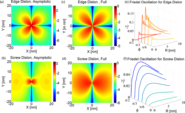
Figure 2. The self-energy of an electron away from a dislocation line with a dislocation core  The ratio between the modulus of the self-energy real part
  and electron energy
  is plotted on the log scale, as a function of 2D coordinate
  for edge (a), (c), (e) and screw (b), (d), (f) dislocations. The self-energy decays in an exponential way away from the dislocation core, indicating a short-range interaction. Compared with simpler asymptotic exponential decay behavior (a), (b), full coupling constants (c), (d) calculations indeed reveal an exotic Friedel oscillation, which is anisotropic and can occur with only single electron at present. This can be seen more clearly on linear scale waterfall plots (e), (f). The much more drastic oscillation for edge dislocation (e) than screw dislocation (f) is caused by dilatation effect and resulting electrostatic potential.
Download figure:
Standard image High-resolution imageThe most prominent feature is that the electron real part of self-energy  shows an anisotropic single-electron energy oscillation behavior as an angle
  with respect to the glide plane (xz plane in figure 1(b)), as shown in figures 2(e) and (f). Since a single dislocation is a 1D defect, the traditional electron density oscillation, namely the Friedel oscillation, is easily pictured as a direct generalization to the 0D point-defect Friedel oscillation [37, 38]. However, what is striking here is that the oscillation here is not an electron density oscillation, but a pattern of electron energy oscillation instead. Such an oscillation can be traced back from equation (34) due to the oscillating Bessel functions in the coupling strength, instead of any artifacts caused by the procedure related to Debye wavevector
  Unlike the traditional Friedel oscillation which occurs only with a bunch of electrons forming an electron liquid, here the energy oscillation can emerge when only one single electron is present. Such an energy oscillation does not indicate that the electron energy will constantly vary when traveling nearby a dislocation core. Under the 1-loop correction (supplementary material D), such an oscillation can be understood as an electron-dislon interaction event taking place at a spatial position r, where an electron emits and reabsorbs a virtual-dislon for once. Due to the extended nature of the quantized dislocation, the interaction event can happen when the electron is away from the dislocation core. Such an interaction event has the effect to change electron energy, according to the 1st formula in equation (40). The amount of the energy change, though, depends on the location r of the interaction event, and is a function of r in an oscillatory instead of monotonic way. Therefore, this energy oscillation behavior is indeed an overall spatial pattern away near the dislocation region, or distribution of the energy change of an electron caused by electron-dislon interaction, instead of a single particle trajectory along which the electron energy keeps changing.
Another feature is that the oscillation caused by an edge dislocation (figure 2(e)) is much more drastic than that caused by a screw dislocation (figure 2(f)). This can be understood from the distinct electrostatic effect contributing to the Friedel oscillation. For an edge dislocation there is a finite inhomogeneous lattice dilatation  leading to a compensating electrostatic potential to reach a uniformly distributed Fermi energy at equilibrium, while for a screw dislocation, the linear elasticity gives no dilatation and hence no electrostatic effect emerges [1]. In order for such an observation, high-resolution, low-temperature scanning tunneling spectroscopy can be performed, where a single electron can be injected from the tip at different positions away from the dislocation core, with its energy derived indirectly from the measured spectroscopies. The observation of the predicted self-energy's single-electron energy Friedel oscillation may provide strong evidence of the existence of the dislon and thereby the quantum nature of crystal dislocations. In fact, a recent simulation indicates the necessity to incorporate the quantization of the crystal vibrational modes in considering the plastic deformation process [39]. The dislon theory may thus serve as an analytical framework to account for the vibrational modes in a dislocated crystal.
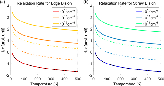
To test the power of this theoretical framework, we compare the relaxation rate  from equation (39) to the well-known semi-classical results as reported in [40]. Despite the different methods, our one-loop result shares an identical prefactor
  and the same temperature dependence
  with the semi-classical relation
  (
( is the number of dislocations) [40], but our method has a stronger capability to compute the position and energy dependence of the relaxation time, for electrons with different energies, at different spatial points. Assuming a roughly averaged dislocation-electron distance
  the comparison (normalized at 1012 cm−2) of the relaxation rate between our theory and the semi-classical theory is plotted in figure 3 and shows very similar trends. Due to the explicit position dependence of the relaxation time
  in our theory, it is not an easy task to compute the total relaxation time
  Without any position dependence, a simple relation based on Matthiessen's rule
  might be a reasonable starting point summing over degenerate electrons. However,
  does not make sense with the presence of multiple dislocations even if they are not interacting with each other, since an election far away from one dislocation may be closer to another dislocation. The relation between the theoretical computable relaxation time
  and the total election-dislocation relaxation time
  remain an interesting open question, however.
Figure 3. Comparison of normalized relaxation rate using classical result [40] (dashed lines) and equation (39) (solid lines).
Download figure:
Standard image High-resolution image
5. Conclusions
In summary, we have developed a fully-quantized theory of crystal dislocations in order to describe the effect of a dislocation on the electronic properties of materials at a many-body level. Upon quantization, a type of effective 1D Bosonic excitation, which we have called the 'dislon', is developed, whose excitation spectra are obtained in closed-form in an isotropic medium. Such a framework allows one to study the classical electron static-dislocation scattering at a full dynamical many-body quantum–mechanical level. This quantum approach is expected to greatly facilitate the study of the effects of non-interacting dislocations on the electrical properties of materials because the effects of an isolated dislon can be incorporated into existing many-body theories without loss of rigor. In fact, the power of a quantized dislocation is not only restricted to the prediction of the electron energy oscillation. Using this approach, it can be shown that a multi-decade—long debate of the nature of the dislocation-phonon interaction-whether a static strain scattering process or a dynamic fluttering dislocation scattering process—shares the same origin as phonon renormalization [35]. What's more, since the dislon is a type of Bosonic excitation, the dislon may also couple 2 electrons to form a Cooper pair, becoming an extra contributor to superconductivity besides a phonon. This may seem counterintuitive since dislocations are defects, which tend to only shorten the electron mean free path and lead to a weakening of superconducting coherence phenomena; yet early experimental evidence did show a sample annealing temperature dependent superconducting transition temperature Tc, whereby different samples having identical stoichiometry but different dislocation densities, and showed a slight increase of Tc under plastic deformation in another experiment [41]. A more profound role of dislocations on superconductivity was suggested as the competition between two different types of interaction based on the dislon theory [28].
Acknowledgments
ML would thank helpful discussions with Hong Liu, and suggestions by Laureen Meroueh, Qichen Song, Zhiwei Ding, Qian Xu, Zhou, Shengxi Huang and Maria Luckyanova. ML, MSD and GC would like to thank support by S3TEC, an EFRC funded by DOE BES under Award No. DE-SC0001299/DE-FG02-09ER46577, and thank the Defense Advanced Research Projects Agency (DARPA) Materials for Transduction (MATRIX) program HR0011-16-2-0041.