


Abstract
We present a new method of constructing a fully robust qubit in a three-level system. By the application of continuous driving fields, robustness to both external and controller noise is achieved. Specifically, magnetic noise and power fluctuations do not operate within the robust qubit subspace. Whereas all the continuous driving based constructions of such a fully robust qubit considered so far have required at least four levels, we show that in fact only three levels are necessary. This paves the way for simple constructions of a fully robust qubit in many atomic and solid state systems that are controlled by either microwave or optical fields. We focus on the NV-center in diamond and analyze the implementation of the scheme, by utilizing the electronic spin sub-levels of its ground state. In current state-of-the-art experimental setups the scheme leads to improvement of more than two orders of magnitude in coherence time, pushing it towards the lifetime limit. We show how the fully robust qubit can be used to implement quantum sensing, and in particular, the sensing of high frequency signals.
Export citation and abstract BibTeX RIS

Original content from this work may be used under the terms of the Creative Commons Attribution 3.0 licence. Any further distribution of this work must maintain attribution to the author(s) and the title of the work, journal citation and DOI.
1. Introduction
The implementation of quantum technology applications and quantum information processing requires a reliable realization of qubits that can be initialized, manipulated, and measured efficiently. In solid state and atomic systems, ambient magnetic field fluctuations constitute a serious impediment, which usually limits the coherence time to several orders of magnitude less than the lifetime limit. Pulsed dynamical decoupling [1–3] has proven to be very useful in prolonging the coherence time [4–11]. However, in order to mitigate both external and controller noise, very rapid and composite pulse sequences must be applied [12–16], which are not easily incorporated into other operations and require a lot of power [17]. Similarly, in continuous dynamical decoupling [17–25], the effect of the controller noise can be diminished by either a rotary echo scheme [26, 27], which is then analogous to pulsed dynamical decoupling, or by the concatenation of several driving fields [28–30], which is limited by the reduction of the dressed energy gap, and results in slower qubit gates. However, a multi-state system enables a different approach. In [31], a fully robust qubit; i.e., a qubit that is robust to both external and controller noise, was realized by the application of continuous driving fields on a specific hyperfine structure. Subsequently, a general scheme for the construction of a fully robust qubit was introduced in [32].
So far, all the continuous driving based implementations of a fully robust qubit have been investigated [32–36] and experimentally realized [31, 37–40] with the application of on-resonance driving fields. This, however, requires at least four energy levels on which the driving fields operate, and hence is not applicable to a three-level system. In fact, together with a three-level system, an additional hyperfine level was considered in [31]. In [34], one of the excited states of the NV-center was used, but necessitated a cryogenic temperature, and in [32] two Λ systems (composed of six states) were employed.
In this paper we show how a fully robust qubit can be constructed by only utilizing a three-level system through the application of continuous off-resonant driving fields. Our method achieves robustness to driving noise, which is the typical problem of continuous dynamical decoupling schemes. Three level-systems are widely available and appear in many atomic and solid state systems, such as trapped ions, rare-earth ions, defect centers, and in particular, the NV-center in diamond. This scheme is applicable to both optical and microwave configurations. The fact that only the three-level system is manipulated facilitates the realization of the fully robust qubit and its integration in the target application. Moreover, the construction by off-resonant driving fields enables the implementation of fast, simple qubit gates. Our scheme is therefore aimed at enhancing the performance of a wide range of tasks in the fields of quantum information science and quantum technologies, and in particular, quantum sensing, where due to the off-resonance construction, our scheme constitutes a novel method for sensing high frequency signals.
2. Fully robust qubit
We start with an explicit definition of a fully robust qubit [32]. Let us denote by  the robust qubit states. In what follows Hd is the (continuous) driving Hamiltonian,
  is the Hilbert subspace of the fully robust qubit, and
  is the complementary Hilbert space, that is,
  . We define the fully robust qubit by (see figure 1)


The first equation ensures that magnetic noise does not operate within the subspace of the fully robust qubit; the noise can only cause transitions between a robust state and a state in the complementary subspace. We assume (by construction) that the energy of all states in  is far from the energy of the states in
  . More specifically, we assume that
  , where
  (
( ) is an eigenvalue of an eigenstate in
  (
( ), is much larger than the characteristic frequency of the noise, as in this case the lifetime T1 would be inversely proportional to the power spectrum of the noise at ν. This ensures that the rate of transitions from
  to
to  due to magnetic noise is negligible.

Figure 1. Fully robust qubit. By the application of continuous driving fields we create a robust qubit subspace. Magnetic noise and power fluctuations of the driving fields do not operate within the robust qubit subspace. (a) Bare states, Hd (driving Hamiltonian). (b) Fully robust qubit (blue), Ω (smallest energy gap between the robust qubit states and non-robust states.
Download figure:
Standard image High-resolution imageThe second equation indicates that the robust states do not collect a relative dynamical phase due to Hd, and are therefore immune to noise originating from Hd. Power fluctuations of the driving fields result in identical energy fluctuations of the robust states.
To summarize, the first equation ensures that the robust states are immune to external noise, while the second equation ensures that the robust states are also immune to controller noise.
3. Fully robust qubit in a three-level system
The rationale for the method is illustrated in figure 2. Driving a three-level system in a Λ configuration with large detunings results in Stark shifts of all three levels. We design the driving fields; i.e., their Rabi frequencies and detunings, in such a way that the new eigenstates are decoupled, in first order, from the external magnetic field (see equation (1)). In addition, up to the second order, two of the eigenstates have an identical Stark shift (see equation (2)); hence, fluctuations in the energy gap between them are mitigated since noise in the driving fields will cause only fluctuations due to the higher order terms of the Stark shifts. Specifically, we consider driving fields in two Λ configurations. In one Λ configuration the driving fields are red detuned and in the second Λ configuration the driving fields are blue detuned. Denote by Ω the Rabi frequency of the driving fields, and by Δ the detuning. The red detuned driving fields, which correspond to (in the interaction picture (IP))

result in the effective Hamiltonian [41]

Similarly, the blue detuned driving fields, which correspond to

result in the effective Hamiltonian

Our construction therefore results in the effective Hamiltonian

whose  and
and  eigenstates have a zero first order Zeeman shift and identical energies. Hence, the two requirements for a fully robust qubit, equations (1) and (2), are fulfilled by the
  and
and  states (with
  ). Viewed in the
  basis, where
  , the red detuned driving fields induce a positive (negative) Stark shift to the
  (
( ) state, while the blue detuned driving fields induce a negative (positive) Stark shift to the
  (
( ) state. The driving fields are therefore tuned such that the total Stark shift of the
  state will be equal to the Stark shift of the
  state (see figure 2).

Figure 2. Fully robust qubit in a three-level system. (a) Two Λ systems are created via the same level with two unequal detunings of opposite signs. (b) The driving fields of the two Λ systems result in Stark shifts of the three levels, here described in the  basis. In the case where the ratio between the red detuning and the blue detuning is equal to 2 (and for the specific values of the Rabi frequencies), the Stark shifts of the
  and
and  states are identical. At the same time, a large energy gap is formed between the
  and
and  states.
Download figure:
Standard image High-resolution imageWe assume a zero-field splitting between the  and
and  states. In case that the
  states are split, due to a static magnetic field, the on-resonance frequencies of the
  and
and  transitions are not identical, therefore, we consider the regime where
  . Hence, each Λ system requires two different (phase-matched) driving fields and, in the case of a microwave implementation (with linear polarizations), corrections on the order of
  are introduced.
4. Robustness
We first analyze the robustness of the scheme to environmental and controller noise, which are extremely crucial to the NV-based implementation, and then refer to possible errors in the general experimental set-up.
With respect to environmental noise, dephasing of the dressed states is caused by two factors. The first source of dephasing is the high order coupling to the external magnetic field. By construction, the first order coupling is eliminated, but higher order terms remain. This can be grasped by moving to the time independent frame of the dressed states. In the lab frame, and in the basis of the bare states, the Hamiltonian of the noise is given by

where B(t) is a randomly fluctuating magnetic field. Moving to the IP with respect to the energies of the bare states, and then moving to the basis of the dressed states, Hnoise is transformed to

We continue by moving to the time independent frame; that is, to the IP with respect to  . This results in

The Stark shifts obtained by the driving fields are accompanied by a small amplitude mixing between the ideal  states (i.e., the exact eigenstates), which means that HnoiseII is further (slightly) rotated to have both diagonal and other off-diagonal terms. However, due to the high detuning of
  , the effect of all of these contributions is negligible. Therefore, the significant effect of the noise is due to the coupling between the
  and
and  states. In the first order, the noise induces a longitudinal relaxation (decay) rate of
  , where SBB is the power spectrum of the noise, and EBD is the energy gap between the
  and
and  states. Hence, a large EBD ensures that the longitudinal relaxation rate is negligible (
 ). In this case, the noise does not induce transitions between the
  and
and  states, but does result in a second order fluctuating phase shift of
  . The resulting dephasing rate is considerably diminished with an increasing EBD (see appendix
  and
and  states via a Raman transition. In case that the
  states are Zeeman sub-levels, this results in an additional mixing term of
  in the effective Hamiltonian of equation (7), and the mixing is of the order of
  . This implies a dephasing rate of
  , which is greatly suppressed by enlarging the Zeeman splitting.
Regarding controller noise, in an ideal construction the (second order) Stark shifts of the  and
and  states are identical and therefore immunity to controller noise is obtained. However, while we can fix the second order Stark shifts to be identical, the fourth order terms might not be negligible, and in this case will introduce an energy gap between the
  and
and  states. Fluctuations of this energy gap, due to driving amplitude noise, can be significantly reduced by either an exact calculation of the fourth order energy shifts, or a numerical search for the point of a non-zero second order shift, which is robust to driving fluctuations5
. In appendix
states. Fluctuations of this energy gap, due to driving amplitude noise, can be significantly reduced by either an exact calculation of the fourth order energy shifts, or a numerical search for the point of a non-zero second order shift, which is robust to driving fluctuations5
. In appendix
For the case of an NV-center in diamond, which we analyzed in detail (see below), our scheme achieves a significant improvement in the coherence time under realistic conditions that take into account both environmental noise and power fluctuations of driving fields.
The robustness of the scheme may also be affected by errors in the experimental set-up. An uncertainty, or a drift, of the static magnetic field,  , shifts the bare
  and
and  states, and therefore introduces two-photon detunings. Compared to the effect of the fluctuating magnetic noise, the dominant effect here is a first order effect. The coupling between the
  and
and  states results in an amplitude mixing and the
  state is modified to
  . Hence,
  inflicts a dephasing rate of
  . This dephasing rate, however, remains negligible as long as the energy gap between the dressed states is much larger than the magnetic field uncertainty; that is,
  . In addition, there can be relative amplitude and relative phase errors between the two driving fields of a Λ system. In both cases, a relative error of ε will introduce an amplitude mixing of
  and an energy shift of
  . For example, a relative amplitude error of ε in the red detuned Λ system introduces (in the IP) the coupling term
  , which results in an amplitude mixing of
  between the
  and
and  states. Since the magnetic noise rotates at the same frequency as this coupling term (see equation (10)) and because there is an amplitude mixing of
  between the
  and
and  states, we have that
  , and hence, the inflicted dephasing rate due to a relative amplitude error of ε is
5. Single qubit gates
In this section we show how protected qubit gates can be implemented and discuss their application for sensing. A  gate can be realized by driving the
  transition on resonance with

Note that while a concatenated on-resonance driving scheme allows for slow gates with  , where
  is the Rabi frequency of the last driving field, our method enables fast gates, where
  is limited solely by the detuning,
  (see figure 3). A
  gate can be realized by introducing a phase shift of
  in the driving frequency with respect to the driving frequency of the
  gate. Alternatively, one can start with a polarization that corresponds to the
  gate, and then add the
  phase shift to get the
  gate. These realizations of
  or
or  gates require two (phase-matched) driving fields, which only couple the
  state to the
  state (similar to the dressing fields). A simpler implementation of the gates can be achieved by employing only one of the driving fields. However, as this driving field couples both the
  and
and  states to the
  state,
  is limited by
  .
.

Figure 3. Single qubit gate and sensing. A single qubit gate in the bare states basis (a), and in the dressed states basis (b). Red (green) arrows correspond to a gate with  (
( ). The green gate enables the sensing of high frequency fields. (c) Control field used for the sensing of low frequency fields via a Raman transition in the bare states basis. (d) The sensing Raman transition in the dressed states basis, where g denotes the sensing field. Dashed arrows in (a) and (c) represent the dressing driving fields.
Download figure:
Standard image High-resolution image6. Sensing
Sensing of high frequency signals is of great importance, especially in the case of classical fields sensing [42, 43], in detection of electron spins in solids [44] and NMR [45]. To the best of our knowledge, to date, dynamical decoupling techniques have not been incorporated in sensing schemes of high frequency signals, which are therefore limited by  . Our scheme enables enhanced sensing of high frequency AC signals, where a signal induces rotations of the fully robust qubit. This can be accomplished by tuning the frequency of the
  transition to the sensing field frequency, as in this case the frequency corresponds to the energy gap between the bare
  and
and  states. Since the sensing sensitivity scales, in the shot noise limit, like
  , for the case of sensing with an NV-center our scheme predicts an improvement of ∼1 order of magnitude in sensitivity.
Sensing of AC signals with lower frequencies can by done by a Raman transition. We assume that the AC signal corresponds to a  operation, which couples the
  and
and  states, and its amplitude is denoted by g. A Raman transition between the
  and
and  states is achieved by adding a control field whose frequency is tuned to match the same detuning as that of the AC signal, so a one-photon detuning is obtained (see figures 3 (c) and (d)). Full oscillation will then be observed whenever
  , where
  is the Rabi frequency of the control field. In this case the sensing sensitivity is limited by the fluctuations of the (dressing) Rabi frequency, Ω, which results in fluctuations of the one-photon detuning, δ. Ideally, the sensitivity scales like
  , where
  is the coherence time induced by the Rabi frequency fluctuations. Note that the sensitivity of low-frequency signal sensing using the bare state scales like
  , while a scaling of
  is obtained by utilizing the
  transition of the dressed states.
7. Implementation with the NV-center in diamond
The electronic ground state of the NV-center is a spin 1 state, where the  states are separated from the
  state by a zero-field splitting of
  [46, 47] (see figure 4(a)). We consider a static magnetic field, which is applied along the NV axis, such that
  GHz (note that a larger Zeeman spitting would result in a better decoupling from the magnetic noise). In this case level-crossing occurs and the energy gaps between
  and
and  correspond to
  and
and  (see figure 4(b)). We assume that to have a good decoupling of the robust qubit and the magnetic noise we need to create an energy gap of
  between the
  and
and  states; hence, we set
  [48, 49]. This implies that the conditions for an ideal construction,
  , are not fully satisfied and therefore the Stark shifts will have contributions from all driving fields as well as from the counter-rotating terms. The Hamiltonian of the system is given by

where  and
and  . By moving to the IP with respect to
  (but not taking the rotating-wave approximation (RWA)), and then moving to the ideal dressed states basis ,
  we obtain
  , from which we calculate, in the ideal dressed states basis, the energy shifts of the dressed states (up to the second order)6
[41]. The energy shifts are given by7
, from which we calculate, in the ideal dressed states basis, the energy shifts of the dressed states (up to the second order)6
[41]. The energy shifts are given by7


In an ideal scenario the terms  would be negligible, and hence, the requirement
  would imply
  .
.

Figure 4. Implementation with the NV-center. Ground state of the NV-center. (a) Without a static magnetic field. (b) With a static magnetic field and driving fields. The ratio of  to
to  is chosen such that robustness to power fluctuations of driving fields is achieved.
Download figure:
Standard image High-resolution imageIn order to achieve an energy gap of  between the
  and
and  states, together with
  , we also set
  . For
. For  , the energy gap between the
  and
and  states, due to the fourth order energy shifts, is
  , which means that driving fluctuations will impose a limitation on the coherence time. We therefore tune the energy shifts to a robust point at which
  , and
, and  (see footnote 5). In this case we have that
  ,
,  , and
, and  .
.
We verified the robustness of this scheme by simulating its performance when the NV spin was subject to magnetic noise and driving fluctuations. We modeled the magnetic noise,  , as an Ornstein–Uhlenbeck process [50, 51] with a zero expectation value,
  , and a correlation function
  . An exact simulation algorithm [52] was employed to realize the Ornstein–Uhlenbeck process, which according to

where n is a unit Gaussian random number. We took the pure dephasing time to be  and the correlation time of the noise was set to
  [53, 54], where the diffusion constant is given by
  Driving fluctuations were also modeled by an an Ornstein–Uhlenbeck process with a zero expectation value. We chose a correlation time of
  , and a relative amplitude error of
  so the diffusion constant is given by
  . Figure 5 presents the outcome of the simulation of the fully robust qubit under the effect of magnetic and driving noise. The plot shows oscillations between the
  states averaged over 200 trials. The oscillations are not symmetric because fast oscillations due to counter-rotating terms at (local) minimum values of P are averaged to zero. The simulation confirmed our estimation of
  , an improvement of more than 2 orders of magnitude in the coherence time, pushing it towards the lifetime limit. Note that the simulation does not take decoherence due to longitudinal spin relaxation (of the bare states) into account, which is given by
  , where
  (since
  , the effect of the noise on the life time of the dressed states is negligible).

Figure 5. Coherence time. Simulation of an NV-center implementation of a fully robust qubit where  μs,
μs,  ,
,  and
and  . The graph is a result of average over 200 trails, and shows oscillations between the
  states. The theoretical dephasing rate is plotted in green and corresponds to a coherence time of
  .
.
Download figure:
Standard image High-resolution imageThe probability of remaining in the initial  state is given by (green line in figure 5)

where


and

 corresponds to the (second order) dephasing due to the coupling between
  and
and  (see appendix
  is the (first order) dephasing rate due to the amplitude mixing between
  and
and  , and
, and  is the dephasing rate due to driving fluctuations, where
  . In our case we estimated that
  Hz,
Hz,  Hz, and the coherence time due to the coupling between
  and
and  alone is
  . In appendix
We used our theoretical model to estimate the achievable coherence times in different scenarios. Figure 6 shows the estimated coherence times for the case of  as function of the correlation time of the noise and for various values of the Zeeman splitting. The parameters chosen for these estimations (see appendix

Figure 6. Lower bound estimation of T2. A theoretical (non-optimized) estimation of the coherence times for the case of  μs as function of the correlation time of the noise and for various values of the Zeeman splitting.
Download figure:
Standard image High-resolution image8. Conclusion
We presented a new method that enables the construction of a fully robust qubit utilizing a three-level system alone. By the application of off-resonance continuous driving fields in a Λ configuration, robustness to both external and controller noise is achieved. We analyzed the NV-center based implementation of the scheme and showed that with current state-of-the-art experimental setups the scheme enables an improvement of more than two orders of magnitude in the coherence time. Moreover, since the scheme allows for fast gates, it is advantageous with respect to on-resonance driving schemes, since more qubit operations in a given T2 time interval can be performed. Our analysis of the NV-center based implementation considered linearly polarized fields. The performance of the scheme is likely to be further improved by the application of circularly polarized fields [55]. This scheme is relevant to many tasks in the fields of quantum information science and quantum technologies, and in particular to quantum sensing of high frequency signals. The utilization of off-resonance driving fields makes the scheme more robust to an inhomogeneous broadening than schemes that use (continuous) on-resonance driving fields, and hence, it is more attractive for ensemble-based sensing. Our scheme is expected to perform even better in the optical regime, where large energy gaps, stronger driving fields, and polarization dependent transitions allow for much smaller mixing amplitudes between the ideal dressed states. Although here we considered the case of a spin 1 system, the scheme is also applicable to systems of half-integer spins. For example, in the case of the calcium ion,  , one could consider a Λ system composed of the
  ,
,  ,
,  states. In this case a fully robust optical qubit can be realized with
  and
and  .
.
Acknowledgments
AR acknowledges the support of the Israel Science Foundation (grant no. 039-8823), the support of the European commission (STReP EQUAM Grant Agreement No. 323714), EU Project DIADEMS, the Marie Curie Career Integration Grant (CIG) IonQuanSense(321798), the Niedersachsen-Israeli Research Cooperation Program and DIP program (FO 703/2-1). This work was [partially] supported by the US Army Research Office under Contract W911NF-15-1-0250. This project has received funding from the European Union as part of the Horizon 2020 research and innovation program under grant agreement No. 667192. FJ acknowledges the support of ERC, EU projects SIQS and DIADEMS, VW Stiftung, DFG and BMBF.
Appendix A:
Here we analyze the dephasing of a strongly driven system. We consider the case of a two-level system (TLS) under a single on-resonance driving and magnetic noise. The Hamiltonian is given by

where B(t) is the random magnetic noise (here in units of frequency). Moving to the IP with respect to  , taking the rotating-wave-approximation (RWA), and moving to the dressed states basis, we get that

In the regime of a strong driving field,  , the time evolution of the dressed states can be simplified by the adiabatic approximation and hence, the dressed states accumulate a phase which is given by

We assume that  is an Ornstein–Uhlenbeck random process [50, 51], which is described by the stochastic differential equation

where  , τ and c are the correlation time and the diffusion constant of the noise, and Wt is a Wiener process. In this case
  is known as the square-root process, or the Cox–Ingersoll–Ross (CIR) process [56], whose stochastic differential equation is given by

Denote the random phase by  . The characteristic function of the square-root process is explicitly given by [56, 57]

where


and we assume that  .
.
We therefore conclude that in the strong driving regime, the probability to remain in the initial equal superposition state of the dressed eigenstates is given by

We numerically verified this by simulating the noise,  , as an Ornstein–Uhlenbeck process with a zero expectation value,
  , and a correlation function
  . An exact simulation algorithm [52] was employed to realize the Ornstein–Uhlenbeck process, which according to

where n is a unit Gaussian random number. We took the pure dephasing time to be  and the correlation time of the noise was set to
  . The diffusion constant was therefore given by
  In figure 7 the pure dephasing (no driving) is plotted. Then, for two values of Ω,
  and
and  we simulated the time evolution of the TLS, which is initialized to
  , the equal superposition of the dressed eigenstates. Figures 8 and 9 show the probability of remaining in the initial state as a function of time. The analytical expression of
  is plotted in green. In addition, we numerically calculated this probability, which by the adiabatic approximation is given by
  . In figures 10 and 11 P is plotted as a function of time and agrees with the analytical expression of
  , which is plotted in green. Increasing Ω increases T2. Indeed, a
  is obtained with a driving of
  MHz respectively. If figure 12 we plot T2 as function of Ω.
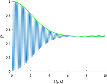
Figure 7. Simulation of pure dephasing with no driving fields.  is plotted in green
  .
.
Download figure:
Standard image High-resolution image
Figure 8. Simulation of the coherence time under a driving of  . Average over 1000 trials.
  is plotted in green.
Download figure:
Standard image High-resolution image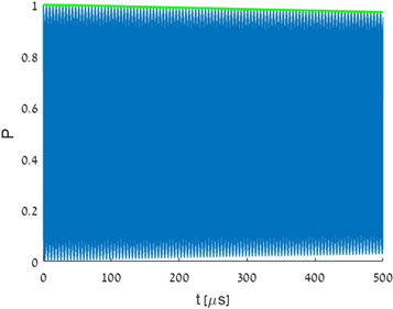
Figure 9. Simulation of the coherence time under a driving of  . Average over 1000 trials.
  is plotted in green.
Download figure:
Standard image High-resolution image
Figure 10. Adiabatic approximation with  . Numerical calculation of
  . Average over 10 000 trials.
  is plotted in green.
Download figure:
Standard image High-resolution image
Figure 11. Adiabatic approximation with  . Numerical calculation of
  . Average over 10 000 trials.
  is plotted in green.
Download figure:
Standard image High-resolution image
Figure 12. T2 as function of Ω. The coherence times where deduced by setting  .
.
Download figure:
Standard image High-resolution imageAppendix B:
The robustness of the scheme to external noise depends on the energy gap between the dressed states, and can, in principle, be improved by increasing both the Rabi frequency of the driving fields and the detuning Δ. As these are limited, an improvement can be achieved by a double-drive, where in the first drive on-resonance driving fields are applied. The energy gap of the dressed states, which are immune to external noise, is now  (compared to an energy gap of
  in the case of a single off-resonance driving) (see figures 6(a) and (b)). Next, we add off-resonance driving fields, which results in an effective
  Hamiltonian of the dressed states, and thus achieves robustness to controller noise as well (see figures 13(c) and (d)). In the IP, and taking the RWA, the Hamiltonian of the on-resonance driving fields is given by

Its eigenstates and eigenvalues are given by  and
and  respectively. Note that all three eigenstates are immune to external noise. In order to construct an effective
  (or
(or  ) driving Hamiltonian of these dressed states, we first need to construct the couplings
  and
and  as building blocks, and then use these for the construction of two off-resonance Λ systems, as in the single-drive scheme (see figure 2). By adjusting the phases of the driving fields, which correspond to the
  and
and  transitions, the coupling
  can be constructed. Moving to the dressed states basis, this results in a
  coupling. Similarly, by adjusting the phases, the
  coupling is achieved, and adding a phased-matched Sz term results in the desired
  coupling. Hence, an effective
  Hamiltonian for the dressed states can now be obtained. Alternatively, it can be shown that the effective Hamiltonian, which in the bare states basis is given by

where  and
and  , results in
  in the dressed states basis, when moving to the dressed states basis and to the IP with respect to
  . Heff can be constructed with off-resonance driving fields, similar to the single-drive construction.

Figure 13. Improving robustness by a double-drive. The first on-resonance driving in the bare states basis (a), and the obtained dressed states (b), which are immune to magnetic field fluctuations. (c) Off-resonance driving fields in the dressed states basis and in the first IP, which result in the effective  Hamiltonian. (d) Doubly dressed states. The Stark shifts of the
  and
and  states are identical.
Download figure:
Standard image High-resolution image
Figure 14. P as function of t.  —first order dephaing rate due to magnetic noise (green),
  —second order dephaing due to magnetic noise (orange), and
  —dephasing rate due to noise in the driving fields (purple). The total probability to remain in the initial state (red) is given by
  (see equation (17)). Gridlines at
  and
and  .
.
Download figure:
Standard image High-resolution imageAppendix C:
In figure 14 we show the effect of the different sources of noise on the coherence time, which together result in  .
.
Appendix D:
Here we give the values of the parameters used in the estimation of T2 in the case of  μs. We assume that in all cases we can find a robust point such that
  (compared to
  of the simulation).
 (GHz) (GHz) |
Ω (MHz) |
 (MHz) (MHz) |
 (Hz) (Hz) |
|---|---|---|---|
| 10 | 60 | 300 | 285 |
| 20 | 60 | 300 | 285 |
| 30 | 75 | 400 | 285 |
| 40 | 85 | 450 | 285 |
| 50 | 100 | 500 | 285 |
Footnotes
- 5
Under a driving fluctuation,
 , there is always a point of the parameters such that the energy fluctuations of the and states are equal, , in the first order in . We assume that we can find a set of values of the parameters which is close enough to this point.
 - 6
Note that since we do not make the RWA, the assumption of a narrow band of frequencies,
, made in [41] does not hold in this case. This, however, does not effect the validity of the calculation. - 7
The energy shifts due to the effective coupling between the
and states are , which is ∼2 orders of magnitude smaller than the leading contributions of the counter-rotating terms of . We therefore neglect these terms in the calculation of the energy shifts.


