Spreading of correlations in exactly solvable quantum models with long-range interactions in arbitrary dimensions

We consider a generic quadratic bosonic Hamiltonian

$$\begin{eqnarray}&&\hat{{ \mathcal H }}=\displaystyle \frac{1}{2}\displaystyle \sum _{{\bf{R}},{{\bf{R}}}^{\prime }}[{{ \mathcal A }}_{{\bf{R}},{{\bf{R}}}^{\prime }}({\hat{a}}_{{\bf{R}}}^{\dagger }{\hat{a}}_{{{\bf{R}}}^{\prime }}+{\hat{a}}_{{{\bf{R}}}^{\prime }}{\hat{a}}_{{\bf{R}}}^{\dagger })+{{ \mathcal B }}_{{\bf{R}},{{\bf{R}}}^{\prime }}({\hat{a}}_{{\bf{R}}}{\hat{a}}_{{{\bf{R}}}^{\prime }}+{\hat{a}}_{{\bf{R}}}^{\dagger }{\hat{a}}_{{{\bf{R}}}^{\prime }}^{\dagger })],\end{eqnarray} \tag{ 1 }$$

where ${\bf{R}}$ and ${{\bf{R}}}^{\prime }$ span the sites of a regular D-dimensional hypercubic lattice of unit lattice spacing. ${\hat{a}}_{{\bf{R}}}$ and ${\hat{a}}_{{\bf{R}}}^{\dagger }$ are, respectively, the annihilation and creation operators at site ${\bf{R}}$, with the usual bosonic commutation relations $[{\hat{a}}_{{\bf{R}}},{\hat{a}}_{{{\bf{R}}}^{\prime }}^{\dagger }]={\delta }_{{\bf{R}},{{\bf{R}}}^{\prime }}$, and the coefficients ${{ \mathcal A }}_{{\bf{R}},{{\bf{R}}}^{\prime }}$ and ${{ \mathcal B }}_{{\bf{R}},{{\bf{R}}}^{\prime }}$ are coupling amplitudes, containing both short- and long-range terms A variety of systems can be described by the Hamiltonian (1). Examples include weakly interacting bosons and spin systems in strongly polarized states, see [51, 52]. Without loss of generality, we write ${{ \mathcal A }}_{{\bf{R}}}=2{h}_{{\bf{R}}}+{{ \mathcal B }}_{{\bf{R}}}$. For simplicity, we assume ${h}_{{\bf{R}}}$ is short range, while the long-range character of interactions is entirely included in the coefficient ${{ \mathcal B }}_{{\bf{R}}}$. More precisely, we assume that it contains a contact interaction term and an algebraic long-range interacting term

$$\begin{eqnarray}&&{{ \mathcal B }}_{R}={ \mathcal U }{\delta }_{R}+\displaystyle \frac{{ \mathcal V }}{{R}^{\alpha }}(1-{\delta }_{R}),\end{eqnarray} \tag{ 2 }$$

where ${ \mathcal U }$ is the on-site contact interaction strength, ${ \mathcal V }$ is the long-range interaction strength, and α is some non-negative constant. Generalization to the case where ${h}_{{\bf{R}}}$ also contains long-range interactions is straightforward.

Assuming translation invariance and parity symmetry, the coefficients ${{ \mathcal A }}_{{\bf{R}},{{\bf{R}}}^{\prime }}$ and ${{ \mathcal B }}_{{\bf{R}},{{\bf{R}}}^{\prime }}$ only depend on the Cartesian inter-site distance $R=| {\bf{R}}-{{\bf{R}}}^{\prime }|$. This condition allows us to write Hamiltonian (1) in momentum space as

$$\begin{eqnarray}&&\hat{{ \mathcal H }}=\displaystyle \frac{1}{2}\displaystyle \sum _{{\bf{k}}}[{{ \mathcal A }}_{{\bf{k}}}({\hat{a}}_{{\bf{k}}}^{\dagger }{\hat{a}}_{{\bf{k}}}+{\hat{a}}_{-{\bf{k}}}{\hat{a}}_{-{\bf{k}}}^{\dagger })+{{ \mathcal B }}_{{\bf{k}}}({\hat{a}}_{-{\bf{k}}}{\hat{a}}_{{\bf{k}}}+{\hat{a}}_{{\bf{k}}}^{\dagger }{\hat{a}}_{-{\bf{k}}}^{\dagger })],\end{eqnarray} \tag{ 3 }$$

where ${{ \mathcal A }}_{{\bf{k}}}$, ${{ \mathcal B }}_{{\bf{k}}}$, and ${\hat{a}}_{{\bf{k}}}$ are the discrete Fourier transforms of ${{ \mathcal A }}_{{\bf{R}}}$, ${{ \mathcal B }}_{{\bf{R}}}$, and ${\hat{a}}_{{\bf{R}}}$, respectively, with the convention

$$\begin{eqnarray}&&{f}_{{\bf{k}}}\equiv \displaystyle \sum _{{\bf{R}}}{f}_{{\bf{R}}}\exp ({\rm{i}}{\bf{k}}\cdot {\bf{R}}),\end{eqnarray} \tag{ 4 }$$

for any field ${f}_{{\bf{R}}}$. The annihilation and creation operators ${\hat{a}}_{{\bf{k}}}$ and ${\hat{a}}_{{\bf{k}}}^{\dagger }$ fulfill the bosonic commutation rule $[{\hat{a}}_{{\bf{k}}},{\hat{a}}_{{{\bf{k}}}^{\prime }}^{\dagger }]={\delta }_{{\bf{k}},{{\bf{k}}}^{\prime }}$ and, due to parity symmetry, the coefficients ${{ \mathcal A }}_{{\bf{k}}}$ and ${{ \mathcal B }}_{{\bf{k}}}$ are real-valued.

Hamiltonian (3) can now be diagonalized using the standard Bogoliubov transformation [53]

$$\begin{eqnarray}&&{\hat{a}}_{{\bf{k}}}={u}_{{\bf{k}}}{\hat{b}}_{{\bf{k}}}+{v}_{{\bf{k}}}{\hat{b}}_{-{\bf{k}}}^{\dagger },\end{eqnarray} \tag{ 5 }$$

where the functions ${u}_{{\bf{k}}}$ and ${v}_{{\bf{k}}}$ can be assumed to be real-valued without loss of generality and to fulfill condition ${u}_{{\bf{k}}}^{2}-{v}_{{\bf{k}}}^{2}=1$ to ensure the commutation relation $[{\hat{b}}_{{\bf{k}}},{\hat{b}}_{{{\bf{k}}}^{\prime }}^{\dagger }]={\delta }_{{\bf{k}},{{\bf{k}}}^{\prime }}$. Then, provided we choose

$$\begin{eqnarray}&&{u}_{{\bf{k}}}=\mathrm{sign}({{ \mathcal A }}_{{\bf{k}}})\sqrt{\displaystyle \frac{1}{2}\left(\displaystyle \frac{| {{ \mathcal A }}_{{\bf{k}}}| }{| {E}_{{\bf{k}}}| }+1\right)}\quad \mathrm{and}\quad {v}_{{\bf{k}}}=-\mathrm{sign}({{ \mathcal B }}_{{\bf{k}}})\sqrt{\displaystyle \frac{1}{2}\left(\displaystyle \frac{| {{ \mathcal A }}_{{\bf{k}}}| }{| {E}_{{\bf{k}}}| }-1\right)},\end{eqnarray} \tag{ 6 }$$

the Hamiltonian takes the canonical form

$$\begin{eqnarray}&&\hat{{ \mathcal H }}={{ \mathcal E }}_{0}+\displaystyle \sum _{{\bf{k}}\ne 0}{E}_{{\bf{k}}}{\hat{b}}_{{\bf{k}}}^{\dagger }{\hat{b}}_{{\bf{k}}},\end{eqnarray} \tag{ 7 }$$

where ${\hat{b}}_{{\bf{k}}}$ and ${\hat{b}}_{{{\bf{k}}}^{\prime }}^{\dagger }$ represent the annihilation and creation operators of a quasi-particle of momentum ${\bf{k}}$, and

$$\begin{eqnarray}&&{E}_{{\bf{k}}}=\mathrm{sign}({{ \mathcal A }}_{{\bf{k}}})\sqrt{{{ \mathcal A }}_{{\bf{k}}}^{2}-{{ \mathcal B }}_{{\bf{k}}}^{2}}=2\mathrm{sign}(2{h}_{{\bf{k}}}+{{ \mathcal B }}_{{\bf{k}}})\sqrt{{h}_{{\bf{k}}}({h}_{{\bf{k}}}+{{ \mathcal B }}_{{\bf{k}}})}\end{eqnarray} \tag{ 8 }$$

is the quasi-particle dispersion relation. The quantity ${{ \mathcal E }}_{0}$ is the zero-point energy, i.e. the energy of the vacuum of quasi-particles. Dynamical stability requires that the quasi-particle energy ${E}_{{\bf{k}}}$ is real-valued, i.e. ${h}_{{\bf{k}}}({h}_{{\bf{k}}}+{{ \mathcal B }}_{{\bf{k}}})\geqslant 0$.

Equations (5), (6), and (8) provide the complete information to determine any equilibrium and out-of-equilibrium properties of the system.

We focus our attention on the out-of-equilibrium dynamical properties of the system induced by a quantum quench. This protocol consists in preparing the system in some initial state $| {{\rm{\Psi }}}_{0}\rangle$ at time t = 0 and let it evolve under the action of some final Hamiltonian ${{ \mathcal H }}_{{\rm{f}}}$. For instance, $| {{\rm{\Psi }}}_{0}\rangle$ may be the ground state of another initial Hamiltonian ${{ \mathcal H }}_{{\rm{i}}}$. Here we assume that ${{ \mathcal H }}_{{\rm{i}}}$ and ${{ \mathcal H }}_{{\rm{f}}}$ are both generic quadratic bosonic Hamiltonians of the form of equation (1) and the quench amounts to an abrupt change of the amplitudes ${{ \mathcal A }}_{{\bf{R}}}$ and ${{ \mathcal B }}_{{\bf{R}}}$ from the values ${{ \mathcal A }}_{{\bf{R}}}^{{\rm{i}}}$ and ${{ \mathcal B }}_{{\bf{R}}}^{{\rm{i}}}$ to the values ${{ \mathcal A }}_{{\bf{R}}}^{{\rm{f}}}$ and ${{ \mathcal B }}_{{\bf{R}}}^{{\rm{f}}}$. Assuming that the quench ${{ \mathcal H }}_{{\rm{i}}}\to {{ \mathcal H }}_{{\rm{f}}}$ takes place on a time scale shorter than any characteristic dynamical time, the time evolution of the system for t > 0 is determined by the equation

$$\begin{eqnarray}&&| {\rm{\Psi }}(t)\rangle ={{\rm{e}}}^{-{\rm{i}}{{ \mathcal H }}_{{\rm{f}}}t}| {{\rm{\Psi }}}_{0}\rangle ,\end{eqnarray} \tag{ 9 }$$

where we set ℏ = 1. Quantum quenches constitute a controlled protocol to study out-of-equilibrium dynamics of correlated quantum systems and are now experimentally realized in ultracold-atom systems [3, 11, 46, 47, 54–56].

The post-quench dynamical properties of the system can be studied via the correlation function of some local observable ${\hat{{\rm{\Sigma }}}}_{{\bf{R}}}$. Here we consider the simplest observable that can be constructed from the local annihilation and creation operators, that is ${\hat{{\rm{\Sigma }}}}_{{\bf{R}}}={\hat{a}}_{{\bf{R}}}+{\hat{a}}_{{\bf{R}}}^{\dagger }$. The corresponding correlation function is then

$$\begin{eqnarray}&&G({\bf{R}},t)=\langle {\rm{\Psi }}(t)| ({\hat{a}}_{{\bf{R}}}^{\dagger }+{\hat{a}}_{{\bf{R}}})({\hat{a}}_{{\bf{0}}}^{\dagger }+{\hat{a}}_{{\bf{0}}})| {\rm{\Psi }}(t)\rangle .\end{eqnarray} \tag{ 10 }$$

For instance, this correlation function is directly connected to spin–spin correlations in the Ising model within linear spin wave theory (LSWT) (see [43, 52, 57] and section 4.1 for details) and to the density–density correlations in the Bose–Hubbard model within mean-field theory, see [53, 58]. Turning to Fourier space and taking the thermodynamic limit it reads

$$\begin{eqnarray}G({\bf{R}},t) & = & \displaystyle \int \displaystyle \frac{{{\rm{d}}}^{D}{\bf{k}}}{{(2\pi )}^{D}}{{\rm{e}}}^{-{\rm{i}}{\bf{k}}\cdot {\bf{R}}}\langle {{\rm{\Psi }}}_{0}| [{\hat{a}}_{{\bf{k}}}^{\dagger }(t){\hat{a}}_{{\bf{k}}}(t)+{\hat{a}}_{-{\bf{k}}}(t){\hat{a}}_{-{\bf{k}}}^{\dagger }(t)+{\hat{a}}_{-{\bf{k}}}(t){\hat{a}}_{{\bf{k}}}(t)\\ & & +{\hat{a}}_{{\bf{k}}}^{\dagger }(t){\hat{a}}_{-{\bf{k}}}^{\dagger }(t)]| {{\rm{\Psi }}}_{0}\rangle \end{eqnarray} \tag{ 11 }$$

in the Heisenberg picture. In order to compute explicitly the correlation function $G({\bf{R}},t)$, we first substitute the particle annihilation and creation operators by their expressions in terms of the quasi-particle ones associated to the final Hamiltonian

$$\begin{eqnarray}&&{\hat{a}}_{{\bf{k}}}(t)={u}_{{\bf{k}}}^{{\rm{f}}}\,{\hat{b}}_{{\bf{k}}}^{{\rm{f}}}(t)-{v}_{{\bf{k}}}^{{\rm{f}}}\,{\hat{b}}_{-{\bf{k}}}^{{\rm{f}}\dagger }(t),\end{eqnarray} \tag{ 12 }$$

found from the inverse of the Bogoliubov transform (5). We then substitute the quasi-particle operator at time t by its expression

$$\begin{eqnarray}&&{\hat{b}}_{{\bf{k}}}^{{\rm{f}}}(t)=\exp (-{\rm{i}}{E}_{{\bf{k}}}^{{\rm{f}}}t){\hat{b}}_{{\bf{k}}}^{{\rm{f}}}(0).\end{eqnarray} \tag{ 13 }$$

We finally use the two Bogoliubov transformations (5) associated to the initial and final Hamiltonians respectively. At the time of the quench, t = 0, they yield

$$\begin{eqnarray}&&{\hat{a}}_{{\bf{k}}}={u}_{{\bf{k}}}^{{\rm{i}}}{\hat{b}}_{{\bf{k}}}^{{\rm{i}}}(0)+{v}_{{\bf{k}}}^{{\rm{i}}}{\hat{b}}_{-{\bf{k}}}^{{\rm{i}}\dagger }(0)={u}_{{\bf{k}}}^{{\rm{f}}}{\hat{b}}_{{\bf{k}}}^{{\rm{f}}}(0)+{v}_{{\bf{k}}}^{{\rm{f}}}{\hat{b}}_{-{\bf{k}}}^{{\rm{f}}\dagger }(0),\end{eqnarray} \tag{ 14 }$$

and

$$\begin{eqnarray}&&{\hat{a}}_{{\bf{k}}}^{\dagger }={u}_{{\bf{k}}}^{{\rm{i}}}{\hat{b}}_{{\bf{k}}}^{{\rm{i}}\dagger }(0)+{v}_{{\bf{k}}}^{{\rm{i}}}{\hat{b}}_{-{\bf{k}}}^{{\rm{i}}}(0)={u}_{{\bf{k}}}^{{\rm{f}}}{\hat{b}}_{{\bf{k}}}^{{\rm{f}}\dagger }(0)+{v}_{{\bf{k}}}^{{\rm{f}}}{\hat{b}}_{-{\bf{k}}}^{{\rm{f}}}(0).\end{eqnarray} \tag{ 15 }$$

We then find the relation

$$\begin{eqnarray}&&{\hat{b}}_{{\bf{k}}}^{{\rm{f}}}(0)=({u}_{{\bf{k}}}^{{\rm{i}}}{u}_{{\bf{k}}}^{{\rm{f}}}-{v}_{{\bf{k}}}^{{\rm{i}}}{v}_{{\bf{k}}}^{{\rm{f}}}){\hat{b}}_{{\bf{k}}}^{{\rm{i}}}-({u}_{{\bf{k}}}^{{\rm{i}}}{v}_{{\bf{k}}}^{{\rm{f}}}-{v}_{{\bf{k}}}^{{\rm{i}}}{u}_{{\bf{k}}}^{{\rm{f}}}){\hat{b}}_{-{\bf{k}}}^{{\rm{i}}\dagger }.\end{eqnarray} \tag{ 16 }$$

This expression allows us to write the correlation function $G({\bf{R}},t)$ as a function of the position ${\bf{R}}$ and of the time t, and the initial quasi-particle operators ${\hat{b}}_{{\bf{k}}}^{{\rm{i}}}$ and ${\hat{b}}_{{\bf{k}}}^{{\rm{i}}\dagger }$. We then calculate the quantum average over the initial state $| {{\rm{\Psi }}}_{0}\rangle$, which we assume to be the ground state of the initial Hamiltonian ${{ \mathcal H }}_{{\rm{i}}}$, defined by ${\hat{b}}_{{\bf{k}}}^{{\rm{i}}}| {{\rm{\Psi }}}_{0}\rangle =0$ for any ${\bf{k}}$. After some straightforward algebra we find that the correlation function can be evaluated in the thermodynamic limit. It reads

$$\begin{eqnarray}{G}_{{\rm{c}}}({\bf{R}},t) & \equiv & G({\bf{R}},t)-G({\bf{R}},0)\\ & = & \displaystyle \frac{1}{2}\displaystyle \int \displaystyle \frac{{{\rm{d}}}^{D}{\bf{k}}}{{(2\pi )}^{D}}{ \mathcal F }({\bf{k}})\left[{{\rm{e}}}^{-{\rm{i}}{\bf{k}}\cdot {\bf{R}}}-\displaystyle \frac{{{\rm{e}}}^{{\rm{i}}({\bf{k}}\cdot {\bf{R}}-2{E}_{{\bf{k}}}^{{\rm{f}}}t)}+{{\rm{e}}}^{{\rm{i}}({\bf{k}}\cdot {\bf{R}}+2{E}_{{\bf{k}}}^{{\rm{f}}}t)}}{2}\right],\end{eqnarray} \tag{ 17 }$$

where

$$\begin{eqnarray}&&{ \mathcal F }({\bf{k}})=\displaystyle \frac{{{ \mathcal A }}_{{\bf{k}}}^{{\rm{i}}}{{ \mathcal B }}_{{\bf{k}}}^{{\rm{f}}}-{{ \mathcal A }}_{{\bf{k}}}^{{\rm{f}}}{{ \mathcal B }}_{{\bf{k}}}^{{\rm{i}}}}{({{ \mathcal A }}_{{\bf{k}}}^{{\rm{f}}}+{{ \mathcal B }}_{{\bf{k}}}^{{\rm{f}}}){E}_{{\bf{k}}}^{{\rm{i}}}}=\displaystyle \frac{{h}_{{\bf{k}}}^{{\rm{i}}}{{ \mathcal B }}_{{\bf{k}}}^{{\rm{i}}}-{h}_{{\bf{k}}}^{{\rm{f}}}{{ \mathcal B }}_{{\bf{k}}}^{{\rm{i}}}}{({h}_{{\bf{k}}}^{{\rm{f}}}+{{ \mathcal B }}_{{\bf{k}}}^{{\rm{f}}}){E}_{{\bf{k}}}^{{\rm{i}}}}.\end{eqnarray} \tag{ 18 }$$

The first right-hand side term in equation (17) is the asymptotic thermalization value while the second right-hand side term is the time-dependent part. The latter contains the information on the spreading of correlations in the system we are interested in.

Before analyzing the dynamical behavior of the correlation function ${G}_{{\rm{c}}}({\bf{R}},t)$ found above, it is worth discussing the divergences that appear in the various terms of equation (17) due to long-range interactions. This is motivated by the known dynamical behavior of short-range systems. For short-range interacting quantum systems the propagation of correlations following a quantum quench exhibits a light-cone structure in its space–time dynamics [17, 18]. It shows up in the form of a linearly increasing horizon, which can be interpreted as being generated by the contribution of the fastest quasi-particles defined by the final Hamiltonian ${{ \mathcal H }}_{{\rm{f}}}$. For that class of Hamiltonians, the velocity defined by the horizon is then expected to be twice the maximum group velocity of the quasi-particles [19]. This is expected to hold in general, including for long-range systems, whenever the post-quench Hamiltonian has excitations with well-defined, finite group velocities. In contrast, sufficiently long-range interactions can make the group velocity diverge and the quasi-particle picture breaks down [43–45, 49, 59] possibly yielding non-ballistic propagation of correlations. Divergences in the energy spectrum, not only in the group velocity, may further affect the dynamics of correlations. When ${E}_{{\bf{k}}}^{{\rm{f}}}$ diverges, at a finite ${\bf{k}}$ value, the space coordinate becomes irrelevant and the associated characteristic time $\tau \sim 1/{E}_{{\bf{k}}}^{{\rm{f}}}$ vanishes. This may yield instantaneous activation of correlations at arbitrary distance and, consequently the breaking of locality. Note that this scenario is not incompatible with the quasi-particle picture, since divergence of the energy ${E}_{{\bf{k}}}^{{\rm{f}}}$ at finite ${\bf{k}}$ implies divergence of the group velocity ${{\bf{V}}}_{{\bf{k}}}={{\rm{\nabla }}}_{{\bf{k}}}{E}_{{\bf{k}}}^{{\rm{f}}}$ and the break-down of the quasi-particle picture.

It is thus expected that the relevant divergences are those of the quasi-particle spectrum, equation (8), and of the quasi-particle group velocity

$$\begin{eqnarray}&&{{\bf{V}}}_{{\bf{k}}}={{\rm{\nabla }}}_{{\bf{k}}}{E}_{{\bf{k}}}^{{\rm{f}}}=\displaystyle \frac{2[2{h}_{{\bf{k}}}{{\rm{\nabla }}}_{{\bf{k}}}{h}_{{\bf{k}}}+{{\rm{\nabla }}}_{{\bf{k}}}({h}_{{\bf{k}}}{{ \mathcal B }}_{{\bf{k}}})]}{{E}_{{\bf{k}}}},\end{eqnarray} \tag{ 19 }$$

of the post-quench Hamiltonian. We further assume that the parameter ${h}_{{\bf{k}}}$ is regular and it admits a linear development ${h}_{{\bf{k}}}\approx h+{{\bf{h}}}^{\prime }\cdot {\bf{k}}$ in the infrared limit. We then obtain the limit expression

$$\begin{eqnarray}&&{{\bf{V}}}_{{\bf{k}}}=\displaystyle \frac{2}{{E}_{{\bf{k}}}}[(2h+{{ \mathcal B }}_{{\bf{k}}}){{\bf{h}}}^{\prime }+h{{\rm{\nabla }}}_{{\bf{k}}}{{ \mathcal B }}_{{\bf{k}}}].\end{eqnarray} \tag{ 20 }$$

Conversely the parameter ${{ \mathcal B }}_{k}$, which, according to equation (2), reads

$$\begin{eqnarray}&&{{ \mathcal B }}_{{\bf{k}}}^{{\rm{f}}}={{ \mathcal U }}^{{\rm{f}}}+{{ \mathcal V }}^{{\rm{f}}}\displaystyle \sum _{{\bf{R}}\ne 0}\displaystyle \frac{{{\rm{e}}}^{{\rm{i}}{\bf{k}}\cdot {\bf{R}}}}{| {\bf{R}}{| }^{\alpha }},\end{eqnarray} \tag{ 21 }$$

may diverge in the infrared limit, depending on the value of the exponent α. The relevant terms are

$$\begin{eqnarray}&&{{ \mathcal B }}_{{\bf{k}}}^{{\rm{f}}}-{{ \mathcal U }}^{{\rm{f}}}\sim \int {\rm{d}}R\ \int {\rm{d}}{\rm{\Omega }}\displaystyle \frac{{{\rm{e}}}^{{\rm{i}}{kR}\cos (\theta )}}{{R}^{\alpha -D+1}}\sim {k}^{\alpha -D}\qquad \mathrm{and}\qquad {{\rm{\nabla }}}_{{\bf{k}}}{{ \mathcal B }}_{{\bf{k}}}\sim {{\rm{k}}}^{\alpha -D-1}\end{eqnarray} \tag{ 22 }$$

in the thermodynamic limit where Ω is the D dimensional solid angle and θ is the azimuthal angle with respect to ${\bf{k}}$. Typical behaviors of the energy and group velocity for various values of α are shown in figure 1.

Zoom In Zoom Out Reset image size

For $D+1\lt \alpha$ (right column in figure 1), both ${{ \mathcal B }}_{{\bf{k}}}$ and ${{\rm{\nabla }}}_{{\bf{k}}}{{ \mathcal B }}_{{\bf{k}}}$ converge to a finite value in the infrared limit. Hence, both the energy and the group velocity are bounded for any value of the momentum ${\bf{k}}$. Note that the maximum group velocity is not necessary at ${\bf{k}}=0$ as for instance in the example shown in the figure.

For $D\lt \alpha \lt D+1$ (central column in figure 1), ${{ \mathcal B }}_{{\bf{k}}}$ is finite but ${{\rm{\nabla }}}_{{\bf{k}}}{{ \mathcal B }}_{{\bf{k}}}$ diverges in the infrared limit. Hence, the group velocity diverges, giving rise to infinitely fast modes, while the energy is finite with a cusp around the origin. Writing ${{ \mathcal B }}_{{\bf{k}}}^{{\rm{f}}}={{ \mathcal B }}_{0}^{{\rm{f}}}+{{ \mathcal B }}_{0}^{{\rm{f}}^{\prime} }| {\bf{k}}{| }^{\alpha -D}$, we find

$$\begin{eqnarray}&&| {{\bf{V}}}_{{\bf{k}}}| \approx \sqrt{\displaystyle \frac{{h}^{{\rm{f}}}}{{h}^{{\rm{f}}}+{{ \mathcal B }}_{0}^{{\rm{f}}}}}\ \displaystyle \frac{(\alpha -D){{ \mathcal B }}_{0}^{{\rm{f}}^{\prime} }}{| {\bf{k}}{| }^{D+1-\alpha }}.\end{eqnarray} \tag{ 23 }$$

For α < D (left column in figure 1), both ${{ \mathcal B }}_{{\bf{k}}}$ and ${{\rm{\nabla }}}_{{\bf{k}}}{{ \mathcal B }}_{{\bf{k}}}$ diverge in the infrared limit. Hence, both the energy and the group velocity diverge. Writing ${{ \mathcal B }}_{{\bf{k}}}^{{\rm{f}}}\approx {{ \mathcal B }}_{0}^{{\rm{f}}}/| {\bf{k}}{| }^{D-\alpha }$, we find the energy

$$\begin{eqnarray}&&{E}_{{\bf{k}}}^{{\rm{f}}}=\displaystyle \frac{2\sqrt{{h}^{{\rm{f}}}{{ \mathcal B }}_{0}^{{\rm{f}}}}}{| {\bf{k}}{| }^{\tfrac{D-\alpha }{2}}}\end{eqnarray} \tag{ 24 }$$

and the velocity

$$\begin{eqnarray}&&| {{\bf{V}}}_{{\bf{k}}}| =\displaystyle \frac{(D-\alpha )\sqrt{{h}^{{\rm{f}}}{{ \mathcal B }}_{0}^{{\rm{f}}}}}{| {\bf{k}}{| }^{\tfrac{D-\alpha +2}{2}}}.\end{eqnarray} \tag{ 25 }$$

As shown in the following section, those various behaviors play a central role in the qualitative space–time behavior of the correlation function.

Consider first the case where both the energy and the group velocity are bounded in the whole Brillouin zone for the quadratic Hamiltonian described in section 2.1. This occurs for algebraically decaying interactions of the type equation (2) with $\alpha \lt D+1$.

To study the evolution of the correlation function, it is worth separating the static and time-dependent components, and rewrite the correlation function (17) as

$$\begin{eqnarray}&&{G}_{{\rm{c}}}({\bf{R}},t)=g({\bf{R}},t)+{g}_{\infty }({\bf{R}},t),\end{eqnarray} \tag{ 26 }$$

where

$$\begin{eqnarray}&&{g}_{\infty }({\bf{R}})=\displaystyle \frac{1}{2}\int \displaystyle \frac{{{\rm{d}}}^{D}{\bf{k}}}{{(2\pi )}^{D}}{{\rm{e}}}^{-{\rm{i}}{\bf{k}}\cdot {\bf{R}}}{ \mathcal F }({\bf{k}})\end{eqnarray} \tag{ 27 }$$

is the asymptotic thermalization value, and

$$\begin{eqnarray}&&g({\bf{R}},t)=-\displaystyle \frac{1}{2}\int \displaystyle \frac{{{\rm{d}}}^{D}{\bf{k}}}{{(2\pi )}^{D}}{ \mathcal F }({\bf{k}})\left[\displaystyle \frac{{{\rm{e}}}^{{\rm{i}}({\bf{k}}\cdot {\bf{R}}-2{E}_{{\bf{k}}}^{{\rm{f}}}t)}+{{\rm{e}}}^{{\rm{i}}({\bf{k}}\cdot {\bf{R}}+2{E}_{{\bf{k}}}^{{\rm{f}}}t)}}{2}\right]\end{eqnarray} \tag{ 28 }$$

is the time-dependent part. The latter contains the relevant time dependence of the correlation function given by the post-quench dynamics. This contribution may be interpreted as the spreading of two counter-propagating beams of quasi-particles, which are represented by the two oscillating functions ${{\rm{e}}}^{{\rm{i}}({\bf{k}}\cdot {\bf{R}}\mp 2{E}_{{\bf{k}}}^{{\rm{f}}}t)}$. Using the stationary-phase approximation, the main contribution to equation (28) is given by the stationary points of the two phase terms, determined by the two equations

$$\begin{eqnarray}&&{{\rm{\nabla }}}_{{\bf{k}}}({\bf{k}}\cdot {\bf{R}}\mp 2{E}_{{\bf{k}}}^{{\rm{f}}}t)=0.\end{eqnarray} \tag{ 29 }$$

They define the separation and time dependent condition

$$\begin{eqnarray}&&\displaystyle \frac{{\bf{R}}}{t}=\pm 2{{\rm{\nabla }}}_{{\bf{k}}}{E}_{{\bf{k}}}^{{\rm{f}}},\end{eqnarray} \tag{ 30 }$$

where the ± sign represents the two directions of the beams. This procedure can be interpreted as selecting the contribution to the correlation function (28) of the modes with a velocity equal to ${\bf{R}}/t$. Since the group velocity ${{\bf{V}}}_{{\bf{k}}}={{\rm{\nabla }}}_{{\bf{k}}}{E}_{{\bf{k}}}^{{\rm{f}}}$ is bounded for $\alpha \lt D+1$, it has a maximum value V_M. Then equation (30) has solutions only for $| {\bf{R}}| /t\leqslant {V}_{{\rm{M}}}$. This defines a ballistic (linear) horizon, that is a 'light cone', in the $| {\bf{R}}| -t$ plane. Its slope gives the 'light-cone' velocity V_lc, defined by

$$\begin{eqnarray}&&{V}_{\mathrm{lc}}=2\mathrm{Max}({V}_{{\bf{k}}}).\end{eqnarray} \tag{ 31 }$$

The presence of a ballistic horizon in the out-of-equilibrium dynamics is thus directly connected to the presence of a finite absolute maximum of the group velocity [17]. Equation (30) can also predict what happens for points outside the 'light-cone'. If $| {\bf{R}}| /t$ exceeds the maximum value $2{{\bf{V}}}_{{\rm{M}}}$, then equation (30) has no solution. In this case the integration over the oscillating functions has no stationary point and the correlation functions is suppressed.

More precisely for $| {\bf{R}}| /t\lt 2{V}_{{\rm{M}}}$ the contribution to the time-dependent part of the correlation function of the modes with parameter ${\bf{v}}={\bf{R}}/t$ is given by the stationary-phase-approximation expression in generic dimension

$$\begin{eqnarray}&&g({\bf{R}},t)\simeq \displaystyle \sum _{\lambda \in {{ \mathcal S }}_{{\bf{v}}}}{ \mathcal W }({{\bf{k}}}_{\lambda })\cos ({{\bf{k}}}_{\lambda }\cdot {\bf{R}}\pm 2{E}_{{{\bf{k}}}_{\lambda }}^{{\rm{f}}}),\end{eqnarray} \tag{ 32 }$$

where the index λ spans the set of solutions of equation (30) for a fixed value of ${\bf{R}}/t$, ${{ \mathcal S }}_{{\bf{v}}}$. The dimension-dependent quantity

$$\begin{eqnarray}&&{ \mathcal W }({\bf{k}})={\left(\displaystyle \frac{2\pi }{t}\right)}^{\tfrac{D}{2}}\displaystyle \frac{{ \mathcal F }({\bf{k}})}{\sqrt{\det { \mathcal L }({\bf{k}})}},\end{eqnarray} \tag{ 33 }$$

where ${{ \mathcal L }}_{D}$ is the determinant of the Hessian matrix of the final dispersion relation ${E}_{{\bf{k}}}^{{\rm{f}}}$, represents the weight associated to each contributing pair of modes. In practice, some of the modes with the velocity ${\bf{R}}/t$ may be insignificant if they have an extremely small weight ${ \mathcal W }({{\bf{k}}}_{\lambda })$ compared to the other modes with the same velocity. This circumstance, however, does not affect the horizon, as long as at least one mode has a significant weight. In the opposite case the effective spreading of correlations may be slower than the expected bound, equation (31) [44].

Let us now turn to the case where the energy is finite but the group velocity diverges due to a cusp in the energy spectrum around ${\bf{k}}=0$. It follows from equation (8) and the discussion of section 2.3 that the dispersion relation of the post-quench Hamiltonian may be written

$$\begin{eqnarray}&&{E}_{{\bf{k}}}^{{\rm{f}}}={E}_{0}+{V}_{0}| {\bf{k}}{| }^{1-\chi }\end{eqnarray} \tag{ 34 }$$

and the group velocity

$$\begin{eqnarray}&&| {{\rm{\nabla }}}_{{\bf{k}}}{E}_{{\bf{k}}}^{{\rm{f}}}| =(1-\chi ){V}_{0}| {\bf{k}}{| }^{-\chi },\end{eqnarray} \tag{ 35 }$$

where $\chi =D+1-\alpha$. An analytic approach is extremely difficult because of the complexity of the computations. In appendix we detail the computation for the case D = 1 and α = 3/2, where an analytic result can be computed. The result involves the explicit computation of the contribution to the correlation function coming from the modes around ${\bf{k}}\approx 0$, where the group velocity diverges.The correlation function scales algebraically in the large ${\bf{R}}$ and t region scales as

$$\begin{eqnarray}&&{G}_{{\rm{c}}}(R,t)\sim \displaystyle \frac{t}{{R}^{3/2}}.\end{eqnarray} \tag{ 36 }$$

Hence, the correlation horizon is algebraic, t ∼ R^β. While this result is found here for a specific case, we show numerically in section 4.2.2 that it is true for all tested values of the dimension D and of the exponent α. The case analyzed in this section gives β = α, as we will see in section 4.2.2 this cannot be generalized to other values of α where in general, we numerically find $\beta \ne \alpha$.

Note that the scaling (36) is slower than ballistic. This is surprising because it may be expected that a divergent group velocity would allow faster-than-ballistic scaling. This idea is also consistent with extended Lieb–Robinson bounds, which are faster-than-ballistic. Our analysis shows that interference effects between the contributing divergent modes strongly affect the correlation front and the known bounds are not saturated. Note that similar behavior was found in 1D spin chains using many-body numerical approaches [43, 44].

Consider finally the case where the quasi-particle energy spectrum (1) diverges. As discussed in section 2.2 this is the case for α < D, owing to the divergence of the Fourier transform of the potential (2). The dispersion relation around k = 0 takes the form

$$\begin{eqnarray}&&{E}_{{\bf{k}}}^{{\rm{f}}}=\displaystyle \frac{{e}_{0}}{{k}^{\gamma }},\end{eqnarray} \tag{ 37 }$$

where ${e}_{0}=2\sqrt{{h}^{{\rm{f}}}{{ \mathcal B }}_{0}^{{\rm{f}}}}$ and $\gamma =\tfrac{D-\alpha }{2}$. Plugging this expression into equation (17) we find

$$\begin{eqnarray}&&{G}_{{\rm{c}}}(R,t)\sim {\int }_{{\rm{\Omega }}}{\rm{d}}{\rm{\Omega }}{\int }_{\epsilon }^{\pi }{\rm{d}}{{kk}}^{D-1+\gamma }{{\rm{e}}}^{{\imath }{kR}\cos (\theta )}[1-\cos (2{e}_{0}{{tk}}^{-\gamma })],\end{eqnarray} \tag{ 38 }$$

the factor k^γ comes from the contribution of the weight ${ \mathcal F }\sim 1/{E}_{{\bf{k}}}^{{\rm{i}}}$. Since the integral is dominated by the low-k components, the upper bound π of the integral is irrelevant. The lower bound $k=\epsilon$ holds for finite-size systems of linear length L and scales as $\epsilon \sim 1/L$. Hence the limit $\epsilon \to 0$ is equivalent to the thermodynamic limit $L\to \infty$. We proceed by expanding the previous expression in powers of R and find

$$\begin{eqnarray}&&{G}_{{\rm{c}}}(R,t)\sim \displaystyle \sum _{n}\displaystyle \frac{{{\imath }}^{n}{R}^{n}}{n!}{\int }_{{\rm{\Omega }}}{\rm{d}}{\rm{\Omega }}{\cos }^{n}(\theta )\underset{\epsilon \searrow {0}^{+}}{\mathrm{lim}}{\int }_{\epsilon }^{\pi }{\rm{d}}{{kk}}^{D-1+\gamma +n}[1+\cos (\tau {k}^{-\gamma })],\end{eqnarray} \tag{ 39 }$$

where we use the dimensionless time $\tau =2{e}_{0}t$. We can then integrate this expression term by term using the transformation $k\to q={k}^{-\gamma }$ and find

$$\begin{eqnarray}&&{\displaystyle \int }_{\tfrac{1}{{\pi }^{\gamma }}}^{{L}^{\gamma }}{\rm{d}}{{qq}}^{-\tfrac{D+2\gamma +n}{\gamma }}[1-\cos (\tau q)]\\ &&\quad =\displaystyle \frac{{E}_{a}(-{\rm{i}}{L}^{\gamma }\tau )+{E}_{a}({\rm{i}}{L}^{\gamma }\tau )-{E}_{a}(-{\rm{i}}\tau /{\pi }^{\gamma })-{E}_{a}({\rm{i}}\tau /{\pi }^{\gamma })}{2{L}^{D+n+\gamma }},\end{eqnarray} \tag{ 40 }$$

where E_a(x) is the exponential integral function of order $a=\tfrac{D+2\gamma +n}{\gamma }$ [60]. In the last expression, the last two terms are bounded and the limit $L\to \infty$ can be taken without any problem after the summation. We thus focus on the first two terms, which contain the diverging energy contributions that will affect locality. In the large R limit, we find

$$\begin{eqnarray}&&\displaystyle \frac{{E}_{a}(-{\rm{i}}{L}^{\gamma }\tau )+{E}_{a}({\rm{i}}{L}^{\gamma }\tau )}{{L}^{D+n+\gamma }}\sim \displaystyle \frac{\sin ({L}^{\gamma }\tau )}{\tau }\displaystyle \frac{1}{{L}^{2\gamma +D}}\displaystyle \frac{1}{{L}^{n}}.\end{eqnarray} \tag{ 41 }$$

Plugging this expression into equation (39), we find

$$\begin{eqnarray}&&{G}_{{\rm{c}}}(R,t)\sim \underset{L\to \infty }{\mathrm{lim}}\displaystyle \frac{\sin ({L}^{\gamma }\tau )}{\tau }\displaystyle \frac{\int {\rm{d}}{\rm{\Omega }}{{\rm{e}}}^{{\imath }\tfrac{R}{L}\cos (\theta )}}{{L}^{2\gamma +D}}.\end{eqnarray} \tag{ 42 }$$

The last equation shows that an algebraic divergence in the quasi-particles spectrum can lead to a signal which appears on a time scale 1/L^γ and it goes to zero in the thermodynamic limit. Note that this time scale is directly connected to the divergence in the energy spectrum with the same exponent γ. This parameter depends on the specific model and interaction decaying. In our case $\gamma =\tfrac{D-\alpha }{2}$ while the same results applies to free-fermion chain with $\gamma =\tfrac{D}{2}-\alpha$. The latter is consistent with the scaling found in [41]. In this regime, the function $\sin ({L}^{\gamma }\tau )/\tau$ gives rise to a contribution of the type $\delta (\tau )$ to the correlation function at any distance. The same expression can be used to obtain the scaling of the value of the correlation function itself as $G({\bf{R}},t)\sim 1/{L}^{\gamma +D}$. Moreover, these expressions show that the dominant contributions to the correlation function carry spherical symmetry despite the underlying lattice geometry. This will be important for our discussion of the correlation front in section 4.3. In the next section we will check all the analytic prediction made in this and in the last section.

Let us first briefly recall the quadratic approximation for the LRTI model

$$\begin{eqnarray}&&{ \mathcal H }=\displaystyle \frac{V}{2}\displaystyle \sum _{{\bf{R}}\ne {{\bf{R}}}^{\prime }}\displaystyle \frac{{\sigma }_{{\bf{R}}}^{z}{\sigma }_{{{\bf{R}}}^{\prime }}^{z}}{| {\bf{R}}-{{\bf{R}}}^{\prime }{| }^{\alpha }}-h\displaystyle \sum _{{\bf{R}}}{\sigma }_{{\bf{R}}}^{x},\end{eqnarray} \tag{ 43 }$$

where ${\sigma }_{{\bf{R}}}^{j}$ with $j\in \{x,y,z\}$ are the local Pauli matrices and $| {\bf{R}}-{{\bf{R}}}^{\prime }|$ is the Cartesian distance between the two sites ${\bf{R}}$ and ${{\bf{R}}}^{\prime }$ on the D-dimensional hypercubic lattice. In order to write Hamiltonian (43) into the quadratic form (1) we use LSWT. We first rotate the reference axes around the free axis y by an arbitrary angle θ. In the rotated frame, the new spin operators read

$$\begin{eqnarray*}&&{\sigma }_{{\bf{R}}}^{x^{\prime} }=\cos \theta \,{\sigma }_{{\bf{R}}}^{x}-\sin \theta \,{\sigma }_{{\bf{R}}}^{z},\quad {\sigma }_{{\bf{R}}}^{y^{\prime} }={\sigma }_{{\bf{R}}}^{y},\mathrm{and}\quad {\sigma }_{{\bf{R}}}^{z^{\prime} }=\sin \theta \,{\sigma }_{{\bf{R}}}^{x}+\cos \theta \,{\sigma }_{{\bf{R}}}^{z},\end{eqnarray*}$$

and the Hamiltonian

$$\begin{eqnarray*}{ \mathcal H } & = & \displaystyle \frac{V}{2}\displaystyle \sum _{{\bf{R}}\ne {{\bf{R}}}^{\prime }}\displaystyle \frac{{\cos }^{2}\theta \,{\sigma }_{{\bf{R}}}^{z^{\prime} }{\sigma }_{{{\bf{R}}}^{\prime }}^{z^{\prime} }+{\sin }^{2}\theta \,{\sigma }_{{\bf{R}}}^{x^{\prime} }{\sigma }_{{{\bf{R}}}^{\prime }}^{x^{\prime} }-\sin \theta \cos \theta ({\sigma }_{{\bf{R}}}^{x^{\prime} }{\sigma }_{{{\bf{R}}}^{\prime }}^{z^{\prime} }+{\sigma }_{{\bf{R}}}^{z^{\prime} }{\sigma }_{{{\bf{R}}}^{\prime }}^{x^{\prime} })}{| {\bf{R}}-{{\bf{R}}}^{\prime }{| }^{\alpha }}\\ & & -h\displaystyle \sum _{{\bf{R}}}(\sin \theta \,{\sigma }_{{\bf{R}}}^{z^{\prime} }+\cos \theta {\sigma }_{{\bf{R}}}^{x^{\prime} }).\end{eqnarray*}$$

We then use the approximate Holstein–Primakoff transformation [52, 57]

$$\begin{eqnarray}&&{\sigma }_{{\bf{R}}}^{z^{\prime} }\approx {a}_{{\bf{R}}}^{\dagger }+{a}_{{\bf{R}}}\qquad \mathrm{and}\qquad {\sigma }_{{\bf{R}}}^{x^{\prime} }=2{{\rm{n}}}_{{\bf{R}}}-1=2{{\rm{a}}}_{{\bf{R}}}^{\dagger }{{\rm{a}}}_{{\bf{R}}}-1,\end{eqnarray} \tag{ 44 }$$

valid for small bosonic occupation number ${n}_{{\bf{R}}}\ll 1$, and expand the Hamiltonian in the form ${ \mathcal H }={\sum }_{n\geqslant 0}{{ \mathcal H }}_{n}$ where every ${{ \mathcal H }}_{n}$ contains exactly n Holstein–Primakoff particle operators among ${a}_{{\bf{R}}}$, ${a}_{{{\bf{R}}}^{\prime }}$, ${a}_{{\bf{R}}}^{\dagger }$, and ${a}_{{{\bf{R}}}^{\prime }}^{\dagger }$. The zeroth-order term is the classical energy

$$\begin{eqnarray*}&&{E}_{\mathrm{cl}}={L}^{D}\left[\left(\displaystyle \sum _{{\bf{R}}\ne {{\bf{R}}}^{\prime }}\displaystyle \frac{V}{2| {\bf{R}}-{{\bf{R}}}^{\prime }{| }^{\alpha }}\right){\sin }^{2}\theta +h\cos \theta \right],\end{eqnarray*}$$

where L^D is the total number of lattice sites. The rotation angle is chosen to minimize the classical energy, which yields θ = π for antiferromagnetic exchange, V > 0. The Hamiltonian computed in the configuration with θ = π then reads

$$\begin{eqnarray*}&&{ \mathcal H }={E}_{\mathrm{cl}}+\displaystyle \frac{V}{2}\displaystyle \sum _{{\bf{R}}\ne {{\bf{R}}}^{\prime }}\displaystyle \frac{({a}_{{\bf{R}}}^{\dagger }+{a}_{{\bf{R}}})({a}_{{{\bf{R}}}^{\prime }}^{\dagger }+{a}_{{{\bf{R}}}^{\prime }})}{| {{\bf{R}}}^{\prime }{| }^{\alpha }}+2h\displaystyle \sum _{{\bf{R}}}{a}_{{\bf{R}}}^{\dagger }{a}_{{\bf{R}}}.\end{eqnarray*}$$

Up to the (irrelevant) energy ${E}_{\mathrm{cl}}-2{{hL}}^{D}$, this Hamiltonian is of the quadratic form (1) with

$$\begin{eqnarray}&&{{ \mathcal A }}_{{\bf{R}},{{\bf{R}}}^{\prime }}=2\,h{\delta }_{{\bf{R}},{{\bf{R}}}^{\prime }}+\displaystyle \frac{V}{| {\bf{R}}-{{\bf{R}}}^{\prime }{| }^{\alpha }}\qquad \mathrm{and}\qquad {{ \mathcal B }}_{{\bf{R}},{{\bf{R}}}^{\prime }}=\displaystyle \frac{{\rm{V}}}{| {\bf{R}}-{{\bf{R}}}^{\prime }{| }^{\alpha }}.\end{eqnarray} \tag{ 45 }$$

The LRTI model is thus of the form discussed in section 2.1 with a parameter ${h}_{{\bf{k}}}=h$ that does not depend on the momentum ${\bf{k}}$. In particular, the dispersion relation ${E}_{{\bf{k}}}=2\sqrt{h(h+{{ \mathcal B }}_{{\bf{k}}})}$ is a monotonous decreasing function of the modulus of the momentum, $k=| {\bf{k}}|$.

In the following, we consider the time-dependent dynamics of the connected spin–spin correlation function

$$\begin{eqnarray}&&{G}_{{\rm{c}}}^{\sigma \sigma }({\bf{R}},t)=\langle {\sigma }_{{\bf{R}}}^{z}(t){\sigma }_{{\bf{0}}}^{z}(t)\rangle -\langle {\sigma }_{{\bf{R}}}^{z}(0){\sigma }_{{\bf{0}}}^{z}(0)\rangle .\end{eqnarray} \tag{ 46 }$$

Using the Holstein–Primakoff transformation (44), this quantity is exactly the connected correlation function defined by equations (10) and (17).

Figure 2 shows the space–time dynamics of the connected spin–spin correlation function ${G}_{{\rm{c}}}^{\sigma \sigma }({\bf{R}},t)$ (see equation (46)) for various values of the exponent α of the long-range exchange term and the different lattice dimensions D = 1, D = 2, and D = 3. The quench is performed by changing the value of V at fixed h in a LRTI model described by Hamiltonian (43). In particular we used h_i = h_f = 2 for almost all the quenches. The only exception is the one with α = 5/2 and D = 3, where we use h_i = h_f = 4 and ${V}_{{\rm{i}}}=1/2\to {V}_{{\rm{f}}}=1/4$ in order to ensure dynamical stability. For these values the dispersion relation ${E}_{{\bf{k}}}$ is always positive and real-valued. Hence, the initial state $| {{\rm{\Psi }}}_{0}\rangle$, i.e. the ground-state of the initial Hamiltonian, is the vacuum of the magnons. For all the studied cases we checked that the condition n_R ≪ 1 is fulfilled allowing the description of the LRTI model by a Hamiltonian  (3). These results are found by exact numerical integration of equation (17) using equation (18) for the LRTI parameters, see equation (45). In figure 2, the complete evolution as a function of the position R and the time t is shown in 1D, while it is plotted along the diagonals ${\bf{R}}=(R,R)$ in 2D and ${\bf{R}}=(R,R,R)$ in 3D. The results show different behaviors depending on the respective values of α and D. For $D+1\lt \alpha$ (right-hand side column in figure 2), the results show clear evidence of a strong form of locality, namely ballistic cone spreading. While the correlations are significant for t > R/V_lc, where V_lc is some velocity, they are instead strongly suppressed for $t\lt R/{V}_{\mathrm{lc}}$. For $D\lt \alpha \lt D+1$, we still find evidence of locality with correlations appearing for t > F(R), where F is some finite-valued function. This behavior is clear in 1D and 2D while, in 3D, finite lattice size effects hardly permits to determine the function F (see details below). For α < D, the numerical data is compatible with locality breakdown and instantaneous activation of the correlations, irrespective of the distance. Still a very thin band with vanishing correlations is visible at short times. It is due to finite-size effects and their scaling actually confirms locality breakdown (see details below).

Zoom In Zoom Out Reset image size

This behavior is qualitatively consistent with the previous analysis for the different regimes. In the following, we discuss the three identified regimes and provide a quantitative comparison between the analytic predictions and the numerical data.

4.2.1. Local regime $(D+1\lt \alpha )$

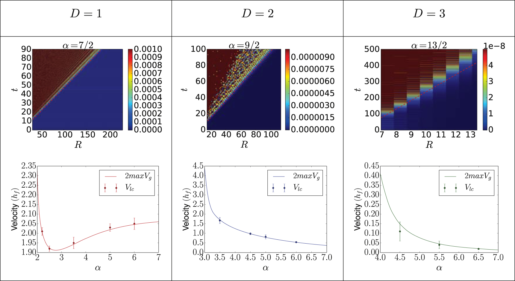
Let us start with the local regime, which corresponds to fast decay of the long-range exchange term, $\alpha \gt D+1$. In this regime, the stationary-phase analysis predicts ballistic spreading of the correlations with a velocity equal to twice the maximum group velocity (see section 3.1). This is confirmed by the complete numerical data. The upper panels of figure 3 show the space–time dynamics of the correlation function, similarly to figure 2, but in contour plot format and with a strong color contrast. It shows a clear ballistic (light-cone-like) behavior of the correlation front in all dimensions. Fitting a linear function, $R={R}_{0}+{V}_{\mathrm{lc}}t$, to the correlation front, we find the light-cone velocity V_lc. The results are compared to the predicted value of twice the maximum group velocity of the final Hamiltonian in the lower panels of figure 3. We find an excellent agreement for all the studied cases within the error bars. The width of the error bars reflects the fact that the leaks outside the light-cone are algebraically decaying, [50], and this makes more complicated to define the exact position of the correlation front. The good quantitative agreement between the numerics and the prediction of equation (31) confirms that the correlation front is mainly determined by the propagation of counter-propagating quasi-particles with the highest velocities, whenever they exist, as predicted by the Cardy–Calabrese scenario [19].

Zoom In Zoom Out Reset image size

4.2.2. Quasi-local regime $(D\lt \alpha \lt D+1)$

In section 3.2 we have demonstrated that the correlation front for α = 3/2 in D = 1 scales as t/R^3/2 but, due to the complexity of the calculation, it has not been possible to extend this result to other cases. It is then important to study the behavior of the correlation horizon for different values of α and different dimensions D. We impose a threshold $\epsilon$ and then we find the first value of time t^⋆ when the correlation function reaches $\epsilon$ for every value of R

$$\begin{eqnarray}&&\bar{G}({t}^{\star },R)=\epsilon .\end{eqnarray} \tag{ 47 }$$

In particular, we consider time-averaged correlation functions, $\bar{G}(t,R)=\tfrac{1}{t}{\int }_{0}^{t}{\rm{d}}\tau {G}_{{\rm{c}}}^{\sigma \sigma }({\bf{R}},t)$, in order to minimize the effects of undesirable small time oscillations.

In the top panel of figure 4 the values of t^⋆ as function of R for a D = 2 system are shown for different values of $\epsilon$ in log–log scale. From these plot, it is clear that there is an algebraic dependence between these two quantities in the large R regime, as suggested by the analytic result for a specific case in section 3.2. We can then interpolate these points with a generic algebraic dependence of the type ${t}^{\star }(R)={t}_{0}^{\star }+m\ast {R}^{\beta }$ for every values of $\epsilon$. The limit $\epsilon \to {0}^{+}$ will give us the correct and $\epsilon$ independent scaling of the horizon ${\mathrm{lim}}_{\epsilon \to 0}\beta (\epsilon )$. This limit can be found in the bottom panel of figure 4 where the values of the fitted parameter β are plotted as function of $\epsilon$ for α = 2.3, and it is possible to see how these results corrects the ones obtained in [44].

Zoom In Zoom Out Reset image size

In figure 5 the values of β as functions of α are plotted for D = 1 and D = 2 systems of different sizes. It is possible to see that $\beta \to 1$ as $\alpha \to D+1$, in agreement with [62], which means that there is a continuous transition between the non-ballistic, $D\lt \alpha \lt D+1$, and the ballistic, $\alpha \gt D+1$, regimes. On the other side, the transition at α = D between the non -local and the non-ballistic regime, is discontinuous. From our data, it is possible to extrapolate the two limits. For D = 1, we find β = 1.52 ± 0.02 for $\alpha \to 1$ and β = 1.01 ± 0.08 for $\alpha \to 2$. For D = 2, we fnd β = 1.56 ± 0.3 for $\alpha \to 2$ and β = 1.1 ± 0.5 and $\alpha \to 3$. This can be explained directly from the expression (17) and from the divergences studied in section 3. In the region α < D the dispersion relation is explicitly divergent, and this leads to the non-local regime studied in section 3.3. For all the values α > D the dispersion relation itself is not divergent and depends continuously on α, which means that in this region the function β has to be continuous too. This motivates the discontinuity of the function β for in α = D and its continuity in $\alpha =D+1$. This last point can be explained naively saying that approaching $\alpha =D+1$ the divergence in the derivative of the dispersion relation disappears, leaving the spectrum without divergences.

Zoom In Zoom Out Reset image size

We now discuss finite-size effects, which are important as we will see. In figure 5, we show a comparison of the values of the parameter β for two 1D systems of different sizes, namely L = 2¹³ = 8192 and L = 2⁶ = 64. In spite of coresponding to system sizes that differ by more than two orders of magnitude, the results are quite close. In particular, they yield $\alpha \to 1$ and $\alpha \to 2$ limits that are consistents within error bars. Nevertheless, the results for the largest system are systematically above those found for the smallest system. In order to get more insight on finite-size effects, we have studied the behavior of β versus the system size for α = 3/2 and D = 1. The results shown on the inset of figure 5 show a systematic increase up to the largest system size we are able to compute. It shows that very large systems are necessary to reach the thermodynamic limit. However, the value of β we find for L = 2¹³ is β ≃ 1.34, which is in fair agreement with the analytic prediction, β = 1.5 within 10%.

4.2.3. Non-local regime ($\alpha \lt D$)

We finally discuss the non-local regime, which corresponds to very weak algebraic decay of the exchange interaction, with α < D. The breaking of locality is apparent in the plots of figure 2 (left column). According to the discussion of section 3.3, it may be attributed to the infrared divergence of the energy spectrum, which corresponds to a vanishing typical activation time of correlations at arbitrary distance in the thermodynamic limit. In order to corroborate the estimate of section 3.3, we may take advantage of finite-size effects. In this case the minimal time scale is provided by the inverse of the maximum energy scale, which corresponds to the momentum k ∼ 1/L. This can be used to obtain an estimate of the system-size dependent activation time

$$\begin{eqnarray}&&\tau \sim \displaystyle \frac{1}{{L}^{\tfrac{D-\alpha }{2}}}.\end{eqnarray} \tag{ 48 }$$

The latter determines the arrival time of the first maximum of the correlation function for large distances. In figures 6(a) and (b) we plot the arrival time τ* of the first maximum of the spin–spin correlation function at a distance equal to half the system size, R = L/2, as a function of L in 1D and 2D. Excellent agreement between the numerical data (points) and the predicted scaling (48) (dashed lines) is found for various values of α < D in both 1D and 2D. These results confirm the predictions of section 3.3. Note that the same scaling can be found from the quasi-particle approach [43]. For power-law spectra as considered here, the group velocity scales as V_k ≃ E_k/k, whose maximum is found for $k\sim 1/L$. Hence the time need to reach half the system size, $L/2$, scales as $1/\max ({E}_{k})\sim 1/{L}^{\tfrac{D-\alpha }{2}}$.

Zoom In Zoom Out Reset image size

Moreover, the analytic approach used in section 3.3 also provides the scaling of the amplitude of the correlation function at t = τ*. It yields

$$\begin{eqnarray}&&{G}_{{\rm{c}}}^{\sigma \sigma }(L/2,{\tau }^{* })\propto \displaystyle \frac{{\tau }^{* }}{{L}^{2\gamma +D}}=\displaystyle \frac{1}{{L}^{\tfrac{3D-\alpha }{2}}}\end{eqnarray} \tag{ 49 }$$

Figures 6(c) and (d) compare numerical data (points) to the analytic prediction above (dashed lines) for the amplitude of the correlation function at R = L/2 and τ*. Good agreement is found in both 1D and 2D. The outcome further confirms the analytic predictions of section 3.3. Note that this result is a direct consequence of the interference between the fastest modes and cannot be found by the simplest independent quasi-particle approach.

In this section we finally discuss the shape of the propagation front during the time evolution of the correlation function. For simplicity, we consider the two-dimensional case but the extension to higher dimensions D is straightforward. In figure 7 the correlation function ${G}_{{\rm{c}}}^{\sigma \sigma }({\bf{R}},t)$, equation (46), for a quench in a D = 2 LRTI system is plotted as function of the position ${\bf{R}}$ at various times t and for different values of the exponent α. In the non-causal regime, α < D, the correlation function is significantly different from zero for every values of ${\bf{R}}$ at any time t. Conversely, in the causal and quasi-causal regimes, for α > D, correlations take a finite time to be activated, which increases as a function of the distance ${\bf{R}}$. For $\alpha \gt D+1$, a sharp edge is visible in the correlations and it evolves ballistically in time. In contrast, for $D\lt \alpha \lt D+1$, the correlation front has a different scaling which is the signature of the quasi-locality. This is consistent with the discussion of section 4.2.

Zoom In Zoom Out Reset image size

Let us now focus on the correlation pattern. For α < D the correlation function is spherically symmetric for large values of R while in the region close to the origin this symmetry is no longer present. This is in perfect agreement with equation (42) which predicts a spherical symmetry of the correlation function in the large R region. For $\alpha \gt D+1$ there is a well-defined correlation front that spreads in the system and its symmetry is spherical despite the presence of the lattice. The symmetry of the front is due to the fact that the maximum group velocity is located very close to ${\bf{k}}=0$, where the spectrum is spherically symmetric (see figure 1). The inner structure of the correlation function is due to the other two local maxima, which are not in the infrared region and whose contribution to the correlation function is not spherically symmetric. This contrasts with the behavior observed for the short-range Bose–Hubbard model, where the maximum group velocity is located at finite ${\bf{k}}$ and gives rise to a non-spherical correlation front in 2D [21]. For the quasi-local regime $D\lt \alpha \lt D+1$ we can use the same arguments used for the other two regimes. The divergence in the velocity located at ${\bf{k}}=0$ is not sufficient to destroy completely locality as discussed in section 3.3 and a sort of locality, called quasi-locality, appears. Still, as for the other two regimes, the modes that dominate close to the horizon are located in the infrared region, where the spherical symmetry of the long-range potential dominates. This determines the spherical symmetry of the correlation function in the large R region. These considerations can be extended straightforwardly to any dimension higher than one because they only rely on the analysis of the symmetries of the energy spectrum and in particular around the point where is located the maximum group velocity that dominates the evolution of the correlation horizon in all regimes.