


Abstract
A notable feature of plasma turbulence is its propensity to retain features of the underlying linear eigenmodes in a strongly turbulent state—a property that can be exploited to predict various aspects of the turbulence using only linear information. In this context, this work examines gradient-driven gyrokinetic plasma turbulence through three lenses—linear eigenvalue spectra, pseudospectra, and singular value decomposition (SVD). We study a reduced gyrokinetic model whose linear eigenvalue spectra include ion temperature gradient driven modes, stable drift waves, and kinetic modes representing Landau damping. The goal is to characterize in which ways, if any, these familiar ingredients are manifest in the nonlinear turbulent state. This pursuit is aided by the use of pseudospectra, which provide a more nuanced view of the linear operator by characterizing its response to perturbations. We introduce a new technique whereby the nonlinearly evolved phase space structures extracted with SVD are linked to the linear operator using concepts motivated by pseudospectra. Using this technique, we identify nonlinear structures that have connections to not only the most unstable eigenmode but also subdominant modes that are nonlinearly excited. The general picture that emerges is a system in which signatures of the linear physics persist in the turbulence, albeit in ways that cannot be fully explained by the linear eigenvalue approach; a non-modal treatment is necessary to understand key features of the turbulence.
Export citation and abstract BibTeX RIS
1. Introduction
Plasma turbulence often retains signatures of the underlying linear eigenmodes in a strongly turbulent state, as found both in theory and simulation [1–6] as well as observations [7–11]. When this is the case, one can predict important features of the turbulence using only the much more-accessible linear information (a notable example is the various quasilinear techniques that have been quite successful in modeling turbulent transport [12–16]). In this context, this paper seeks to characterize and quantify the ways in which nonlinear phase-space structures are connected to the underlying linear eigenmodes (stable and unstable) in a simple gyrokinetic turbulent system.
This question of eigenmodes is particularly interesting in plasma turbulence because it involves extra degrees of freedom in phase space with respect to its neutral fluid counterpart. These extra degrees of freedom may encompass a full multi-dimensional velocity space in kinetic systems, or, simply, multiple fields in the case of plasma fluid models. Various approaches—notably, (1) spectral representations of velocity space, and (2) decompositions—have been applied to understanding this high-dimensional plasma turbulence.
Spectral representations (Hermite polynomials and Bessel functions, for example) for velocity space [17–28] have been used to conceptualize velocity space in terms of scales. Many phenomena fundamental in turbulence theory (like energy injection, transfer, and dissipation) are manifest in the full phase space—i.e., in velocity space scales in addition to real space scales.
The decomposition approach was first applied in plasma fluid systems [29–32], where the complexities of turbulent transport and saturation were studied by projecting the fluctuations onto a basis defined by the underlying linear eigenmodes [29]. This revealed that damped eigenmodes are almost universally excited in these systems [31], defining a novel turbulent scenario that has, in contrast with the Kolmogorov picture, little, if any, scale separation between the scale ranges of energy drive and dissipation. This damped eigenmode approach has been extended to gyrokinetic systems [3, 33–37, 39], where a large class of damped eigenmodes are excited and, similarly, dissipate substantial energy at large scales. It is observed, however, that beyond a small number of modes, this eigenmode basis may not be particularly efficient at capturing the nonlinear state [3]. Moreover, the non-orthogonality of the gyrokinetic linear eigenmodes can make eigenmode decompositions conceptually unwieldy.
A complementary approach uses singular value decomposition (SVD) [33–37, 39] to project the distribution function on an optimal orthogonal basis. These basis functions (SVD vectors) can be used to calculate the unique contribution of various structures to quantities like transport fluxes, energy injection, dissipation, and nonlinear energy transfer. In spite of its clear strengths, the SVD suffers from the fact that, although the SVD vectors represent the optimal basis, we are often left with little intuition regarding the physical origin or underlying nature of this optimal basis. Moreover, due to the fact that the SVD structures must be extracted from existing data, their predictive utility is marginal.
In this work, we add a new aspect to this exploration of plasma phase-space dynamics by linking the linear eigenvalue approach to the SVD approach using pseudospectra [41, 42]. Pseudospectra provide a more nuanced picture of the properties of a linear operator by characterizing its response to perturbations (inherent in any realistic system). This identifies not simply the points in the complex plane that satisfy the eigenvalue equation, but additionally sketches the regions of the complex plane that are close to being eigenvalues and consequently correspond to structures that may be preferentially excited in the nonlinear state. In the spirit of pseudospectral concepts, we propose a novel procedure for quantifying a connection between SVD structures and the linear operator, associating a complex number, which we call the nonlinear pseudo-eigenvalue (NPEV), with each SVD structure. This technique retains both the strong advantages (optimality and orthogonality) of the SVD approach and the intuitive value of the eigenmode picture, effectually endowing the SVD structures with a 'personality' [42].
The course of analysis outlined above is applied to a simple, paradigmatic turbulent system—slab ion temperature gradient (ITG)-driven turbulence described by a reduced gyrokinetic model [25]. This system, which was previously studied in detail in the aforementioned framework of spectral velocity space representations [24, 25], includes linear eigenmodes similar to those familiar from earlier work on fluid models [29] (e.g., ITG modes and drift waves (DWs)), but also kinetic modes representing Landau damping. This work serves to characterize how these familiar ingredients, which underly many basic plasma systems, are manifest in a nonlinear turbulent state.
As it turns out, the SVD structures have certain clear connections with the underlying linear eigenvalue spectra, but also subtle and surprising links with the pseudospectra that could not be inferred from the eigenvalue approach. Moreover, structures are also identified that appear to be intrinsically nonlinear creations having no clear connection with the linear operator.
The value of this work is twofold. First, we present new techniques that elucidate fundamental properties of phase-space turbulece. Second, these insights may find applications in facilitating or refining reduced modeling of turbulent transport (quasilinear models, for example) by identifying the important structures of the turbulence and their relation to the linear eigenmodes.
Following this introduction, the model and corresponding energetics are described in section 2. The remainder of the paper follows an arc progressing from pure linear (section 3) to psuedo-linear (section 4) and finally to fully nonlinear (section 5), where the NPEVs are introduced. We conclude with a summary and discussion in section 6.
2. Reduced gyrokinetic model and energetics
2.1. Model
This study uses the DNA code [24, 25], which solves a reduced gyrokinetic model in an unsheared-slab using a Hermite representation

for parallel velocity space, where Hm(x) is the mth order Hermite polynomial. Hermite polynomials were shown empirically to be an efficient representation of velocity space in gyrokinetic simulations in [43]. Their use in this work was inspired, in particular, by earlier demonstrations of their utility in calculating linear eigenmode spectra [44, 50].
The gyrokinetic equations are integrated over perpendicular velocity space, retaining an approximation of finite-Larmour-radius effects by replacing gyroaverage operators with  (valid for
  [45]). The model includes density and temperature gradients and collisions via a Lenard–Bernstein collision operator [46]. These ingredients produce the linear dynamics of interest for this work, namely temperature gradient driven instabilities, DWs, Landau damping and phase mixing, and collisional dissipation.
The evolution equation for the Hermite moments is

where  is the perturbed (i.e. deviation from Maxwellian) ion distribution function, ni0 is the ion density, R is a macroscopic scale length, vti is the ion thermal velocity, m denotes the order of the Hermite polynomial, t is time,
  is the normalized ITG scale length,
  is the normalized inverse density gradient scale length, ky is the Fourier wavenumber for the direction perpendicular to both the direction of the background gradients
 ![$[x\to {k}_{x}]$](https://content.cld.iop.org/journals/1367-2630/18/7/075018/revision1/njpaa3297ieqn6.gif) and the coordinate aligned with the magnetic field
and the coordinate aligned with the magnetic field ![$[z\to {k}_{z}]$](https://content.cld.iop.org/journals/1367-2630/18/7/075018/revision1/njpaa3297ieqn7.gif) . The perpendicular wavenumber is
. The perpendicular wavenumber is  ,
,  is the gyro-averaged electrostatic potential, Te0 is the background electron temperature, e is the elementary charge, and ν is the collision frequency. Hermite polynomials are, conveniently, eigenvectors of the Lenard–Bernstein collision operator:
![$[(1/2){\partial }_{v}+v]\to \nu m$](https://content.cld.iop.org/journals/1367-2630/18/7/075018/revision1/njpaa3297ieqn11.gif) . Time quantities are normalized to
. Time quantities are normalized to  , the perpendicular directions are normalized to the ion gyroradius
  , the parallel direction is normalized to R, the potential is normalized to
  , and the distribution function is normalized to
  . We employ the adiabatic electron approximation, making electrostatic potential directly proportional to the zeroth-order Hermite polynomial as determined by

where τ is the ratio of the ion to electron temperature, and  , with I0 the zeroth order modified Bessel function.
2.2. Energetics
One advantage of the Hermite representation is the elegant form taken by the energy equations, as described in detail in [25]. Here we note simply that the free energy

is composed of an electrostatic part  and an entropy part
  . In this system, Landau damping is a conservative process that transfers energy from the former to the latter (i.e. from waves to particles) via the term

The net sources and sinks are, respectively, the gradient drive

which is proportional the the heat flux, and the collisional dissipation

which is proportional to the collision frequency ν and the Hermite number m, so that the total energy  evolves according to

The quantities Q/E and C/E (having units of inverse time) represent the rate at which energy is injected or dissipated and will be called the drive and collisional growth rates, respectively. As an illustration, the sum  calculated from a linear eigenvector is equal to twice the linear growth rate (since the quantities are quadratic). These drive and collisional growth rates will be used extensively to characterize linear eigenmodes and SVD structures.
3. Linear eigenmode spectra
In this section we outline the linear eigenmode spectra produced by the various terms in our model. The matrices shown below represent the Hermite-based linear gyrokinetic operator defined in equation (2), so that each row corresponds to a different Hermite moment. This operator can be decomposed as

where  defines the Landau damping and phase mixing terms

and  is the factor that translates between
  and ϕ.
  defines the terms arising from background density and temperature gradients
and  is the collision operator

The eigenvalue spectra associated with different combinations of these operators are shown in figure 1. These spectra are based on eigenvalue solutions of the linear operators defined above using 64 Hermite moments (see [24, 25, 50] for extensive discussion of the numerics underlying both the linear and nonlinear results in this paper). An initial value treatment of the operator  produces the well-known Landau solution [47]—low-order moments that decay in time with damping rates defined by the Landau roots. In contrast, the corresponding eigenvalue problem produces the Case–Van-Kampen modes—a continuum of undamped eigenvalues with singular eigenvectors [48, 49]. Any smooth initial condition will project onto a complete [48, 49] basis of Case–Van-Kampen modes, which then phase mix and reproduce the decay of the low-order moments identified with the initial value treatment. The discretized version of the Case–Van-Kampen spectrum is shown in figure 1(A).
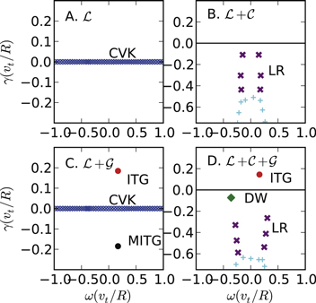
Figure 1. Linear eigenvalue spectra for the wave number kx = 0,  ,
,  for a linear operator that includes only Landau damping (A), Landau damping and collisions (B), Landau damping and gradient terms (C), and the full operator including Landau damping, collisions, and gradient drive (D).
Download figure:
Standard image High-resolution imageA collision operator is a singular perturbation to the system, which unifies the eigenvalue and initial value approaches [44]; even for an infinitesimal value of the collision frequency, the eigenvalues of the combined operator  collapse on the Landau roots, as seen in figure 1(B) (the purple x'(s) are the Landau roots and the cyan + symbols are numerical modes produced by the necessary truncation in Hermite space). The eigenvectors, which were singular (i.e., involve delta functions in velocity space) in the collisionless case, become precisely sharp enough in velocity space to compensate for the smallness of the collisionality. Reference [50] shows that any velocity space derivative of even order is sufficient to reproduce this qualitative behavior. See [51] for an earlier demonstration of a singular perturbation resolving a continuum of singular eigenmodes in the context of a kinetic system describing shear Alfven waves.
The combination  produces the spectrum shown in figure 1(C). The gradient terms give rise to an unstable ITG mode and its complex conjugate, which we will call the mirror ion temperature gradient (MITG) mode. The MITG mode is stable by virtue of an opposite
  cross phase (i.e., negative heat flux Q) with respect to the ITG mode. This combination of operators has been studied in detail in [50], where it was shown that the gradient terms add several discrete roots to the continuous Case–Van-Kampen spectrum, including an undamped DW (which, while present in figure 1(C), is not distinguishable from the Case–Van-Kampen spectrum). This combination of an ITG mode an MITG mode and a marginally stable DW has been studied in a fluid model in [29].
The spectrum of the entire operator  retains features from other spectra discussed as seen in figure 1(D). The ITG mode, which is smooth in velocity space, is relatively unchanged by the addition of the collision operator. The Landau roots are also retained in the presence of gradients, albeit shifted slightly to stronger damping rates. The DW (green diamond) becomes weekly damped, and is now discernible from the Case–Van-Kampen continuum. This mode can be classified as a collisionally stabilized electron DW. It is always stable, with stronger damping at higher kz and lower
  , although its real frequency scales with
  . Due to the fact that it arises from the ITG dispersion relation, it can be viewed as a relative simultaneously of the stable mode in [52] and the neutrally stable mode in [29].
Surprisingly, the MITG mode is no longer an eigenvalue when all terms are included in the linear operator. Intuition would suggest that it would be modified in a manner similar to the ITG mode (i.e., very weakly), but the addition of a collision operator eliminates it entirely from the spectrum. We will return the MITG mode in the context of pseudospectra later in the paper.
The results outlined above are summarized in table 1, which shows the combinations of operators that produce the modes of interest along with a final column previewing the nonlinear conclusions discussed below (section 5).
Table 1. Summary of the scenarios in which the modes of interest are manifest. ITG modes and DWs are present whenever there are driving gradients. As expected, CVK (Case–Van-Kampen modes) are only observed in the absence of collisions. Landau roots (LR) are seen only in collisional linear spectra but are not seen in the nonlinear turbulence. MITG (mirror ITG) modes are, surprisingly, absent from the collisional spectra but reappear in the nonlinear fluctuations, a feature that can be explained by the properties of the pseudospectra.

|

|

|

|

|
|
|---|---|---|---|---|---|
| ITG | X | X | X | ||
| DW | X | X | X | ||
| MITG | X | X | |||
| LR | X | X | |||
| CVK | X | X |
The drive and collisional growth rates for several of the eigenmodes of the full operator are shown in figure 2 (ordered by decreasing growth rate). The ITG mode has a large gradient-drive growth rate due to a positive  cross-phase and a small collisional damping rate due to its smooth velocity space structure (i.e. the eigenmode peaks at low order Hermite numbers). The DW has a similar smooth velocity space structure and also a weak gradient drive. The remaining Landau roots have virtually negligible gradient drive but become increasingly strongly damped due to their increasingly fine-scale velocity space structure.
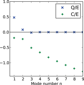
Figure 2. The values of drive growth rates Q/E and collisional growth rates C/E for a series of eigenvectors similar to those corresponding to the eigenvalues shown in figure 1(D). The eigenvectors are labeled in order of linear growth rate so that the first mode is ITG, the second is DW, etc. The growth rates of the modes are equal to  .
.
Download figure:
Standard image High-resolution imageIn this section we have seen that the linear operator for our kinetic slab-ITG model produces various modes familiar from both fluid and kinetic theory: the ITG mode, the MITG mode, a marginally stable DW, and Landau roots. The question is how these modes are manifest in a nonlinear setting. Since the operator is non-Hermitian, the eigenvectors are allowed to be non-orthogonal, and the degree of non-orthogonality of the eigenvectors will be an important factor in how these modes are manifest. In the next section we approach this question in the context of pseudospectra.
4. Pseudospectra
Due to the non-Hermiticity of the operators discussed in the previous section, we may expect that structures observed in a perturbed system may differ significantly from the modes identified above. In this section we address this question by constructing pseudospectra of the kinetic linear operator described above (for other applications of pseudospectra and related non-modal techniques in plasma physics see [53–60]).
4.1. Introduction to pseudospectra
Pseudospectra have been popularized in fluid dynamics by the realization that nonlinear behavior often differs drastically from linear expectations when the linear operators are highly nonorthogonal. A prominent example is high-Reynolds-number Poiseuille flow, which becomes unstable far below the linear critical Reynolds number and does so in a manner that is consistent with the pseudospectra but very different from the linear spectrum [41]. In contrast, our motivation for this work is to find connections—which may be absent in the eigenvalue problem—between the linear operator and the nonlinearly excited structures.
Pseudospectra account for the fact that regions of the complex plane that are far removed from actual eigenvalues may be eigenvalues when the linear operator is subject to even very small perturbations. Definitions of the pseudospectrum rely on the resolvent of the operator  , where A is the operator, I is the identity matrix, and z is a complex number. If z is an eigenvalue then zI − A is singular and
  is infinite. We reproduce below three equivalent (with some restrictions [42]) definitions of the
  -pseudospectrum from [42], each of which has a particular relevance for this work. The
  -pseudospectrum
  is defined as isocontours of
  in the complex plane such that the resolvent is larger than a given value:

The  -pseudospecturm can also be defined in terms of perturbations to the operator:


where  represents an arbritrary deviation from from A, and Λ is the eigenvalue spectrum. Such a deviation could represent, for example, the nonlinear term in the equations.
Another definition relates to the SVD of zI − A,

where  is the smallest singular value of the SVD of zI − A. This definition is useful because it defines a simple method for calculating pseudospectra numerically. It also identifies the right singular vector corresponding to
  as the most-resonant vector, i.e., the vector that is closest to being an eigenvector at the point z in the complex plane. This most-resonant vector will be called the pseudo-eigenvector below.
4.2. Pseudospectra of the kinetic slab ITG operator
Pseudospectra of the kinetic slab ITG operator are shown in figure 3 for a wavenumber representative of the strongly unstable region of k-space. The contours are closely nested around the ITG mode, indicating that it is quite orthogonal to the remaining eigenvectors. The pseudospectra also distinguish (to a lesser degree) the DW ( and
and  ) from the remaining eigenvalues. The region surrounding the Landau roots contains only pseudospectra corresponding to very small values of
  . This is an indication that the eigenvectors corresponding to the Landau roots are highly nonorthogonal and any complex number in this region is close to being an eigenvalue. We would thus expect that structures arising in the nonlinear turbulence may not be easily identifiable with individual eigenvalues in this region of the complex plane.
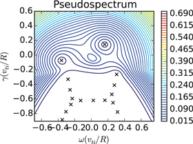
Figure 3. Pseudospectra of the full linear operator for the wave number  ,
,  ,
,  . Note that the contours are closely nested around the ITG mode, and, to a lesser degree, around the DW. The lower portion of the complex plane includes only very low-ε pseudospectra, indicating that complex numbers in this region are all very close to being eigenvalues.
Download figure:
Standard image High-resolution imageSince pseudospectra reflect the non-orthogonality of an operator, we note here that Landau damping represents a violation of Hermiticity. This is readily identified in the non-symmetric term in the matrix  defined in equation (10), which produces the transfer of energy from waves to particles (i.e. Landau damping—quantified by
  in equation (5)). We thus expect that as kz increases and Landau damping becomes stronger, the pseudospectral contours will become increasingly distorted. An example is shown for a high kz wavenumber in figure 4, where it is seen that the ITG mode (now stable) is embedded in elongated contours that no longer separate it from the lower region of the complex plane. Figure 5 shows the deviation of linear growth rates from the nearest point (vertically displaced—i.e., the nearest point with the same frequency) on the
  pseudospectrum as a function of kz for both the ITG mode and the DW. In both cases the deviation increases with kz, indicating that less-damped regions of the complex plane become increasingly accessible. This suggests (1) that the structures that arise in the nonlinear turbulence may deviate strongly from linear expectations for such parameters where Landau damping is expected to be important, and (2) that the nonlinear structures may be substantially less damped than expectations from the linear growth rates.
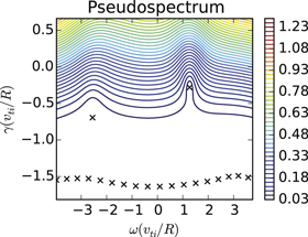
Figure 4. Pseudospectra of the full linear operator for the wave number  ,
,  ,
,  . Contours become increasingly distorted as kz increases (compare with figure 3).
Download figure:
Standard image High-resolution image
Figure 5. The linear growth rates of the ITG and DW modes along with the distance from each to the  contour (vertically displaced). The distance increases as kz increases, suggesting that nonlinear excited modes may deviate more strongly from their linear counterparts as kz increases.
Download figure:
Standard image High-resolution image5. Nonlinear phase space structures
We transition now from linear (and pseudo-linear) physics to fully developed nonlinear turbulence. The nonlinear simulation analyzed here is very similar to those described in detail in [24, 25], to which the reader is referred for numerical details. The collision frequency is  and the normalized gradient scale lengths are
  and
and  (sufficient for a robust ITG instability). [24, 25] describe a transition from a system with predominantly small-scale dissipation to one with predominantly large-scale dissipation depending on the relative driving gradients and collision frequencies. The simulation analyzed here lies firmly in the large-scale dissipation regime so that the subdominant modes described below have a large impact on the total energy balance. In order to allow for analysis of phase space structures, the entire distribution function was output every 50 time steps throughout the simulation.
5.1. SVD analysis
SVD is applied to the turbulence in the following manner: for a given  , the distribution function
  is defined by its dependence on m and t, making it amenable to decomposition of the form
  , where all amplitude information is found in
  , m and t dependence has been separated into
  m p and
  , respectively, and N is the number of elements in the SVD decomposition (minimum of the number of time points and the number of Hermite moments). An SVD produces these ingredients in the form of singular values
  , and orthonormal left and right singular vectors (
 n p and
  , respectively). Moreover, the SVD produces an optimal decomposition in the sense that more energy
  is captured by a truncated SVD decomposition than by any other possible decomposition with the same truncation rank.
The left singular vectors  should then be considered the optimal structures for describing the turbulent phase space, and, having the same form (i.e., dependence only on m) as their linear counterparts (linear eigenvectors or pseudo-eigenvectors), can be compared directly. Using the turbulent distribution function, SVDs were constructed for each wave vector in the simulation. With this optimal decomposition in hand, the remaining challenge is extracting useful information about the turbulence.
5.2. Nonlinear pseudo eigenvalues
We now have three different lenses—linear, pseudospectral, and SVD—through which we can extract and/or interpret nonlinear phase-space structures. Each lens has its distinctive advantages and disadvantages. The linear eigenvalue problem is intuitive and familiar from the historical literature. However, as the pseudospectral approach unveils, the linear eigenmodes may have little to do with what is actually observed in a realistic system. The pseudospectral techniques provide a more nuanced picture of the linear operator, but remain nebulous in other ways, making no certain prediction of the structures that will be excited in the nonlinear turbulence. The value of the SVD is clear—a delineation of the quantifiably most important structures and the manner in which they combine to represent the turbulent fluctuations. However, aspects of the SVD structures may remain as inscrutable as the underlying turbulence from which they are extracted unless further work is done to make connections with meaningful concepts with respect to the turbulence. In this section we describe just such a technique that links all three approaches, revealing patterns in the phase space structures that would be invisible to more conventional analyses.
We start with an SVD decomposition and, in the conceptual spirit of pseudospectra, construct NPEV for each SVD structure as follows. The proximity of an SVD structure to being an eigenvector for a prospective eigenvalue z is given by the quantity

where A is the linear operator. We define the NPEV for a given SVD structure to be the point in the complex plane where  is minimized. An authentic eigenvector would, for example, identify its eigenvalue as the location in the complex plane where
  . We note the connections between this calculation and the calculation of pseudo-spectra; both treatments explore the complex plane for regions of special significance to the linear operator. Whereas the pseudo-spectral technique finds such regions for arbitrary vectors, the NPEV procedure finds points unique to a given vector that optimally represents the turbulent system. As will be outlined below, this procedure extracts some surprising and subtle features that link the linear, pseudo-linear, and SVD analyses.
Figures 6–8 show plots for a series of wave numbers representing the peak energy-containing scales (note that as ky increases, the energy peaks at progressively larger values of kz, roughly consistent with the concept of critical balance [61], which was identified in this system in [24, 25]). These figures encapsulate the main conclusions of this work, synthesizing all three analyses—eigenvalues, pseudospectra, and NPEV. In panel (A), the black x'(s) denote the linear eigenvalues and the contours denote the pseudospectra. The NPEVs are shown as colored symbols, whose color (log scale) denotes the singular value (i.e., average amplitude) of the corresponding SVD structure. The lower panels (B)–(D) show additional information about the SVD structures. The SVD modes are ordered by their singular values, while the symbol shapes denote this ordering and serve to make the connection with the NPEVs in panel (A). Panel (B) shows the drive (Q/E) and dissipation (C/E) growth rates of the structures, panel (C) shows the net contribution to energy balance for each mode (average Q + C), and panel (D) shows the minimized  (the degree to which the SVD structure approximates an eigenvector).

Figure 6. The linear eigenvalues (black x's), pseudospectra (contours), and nonlinear pseudo-eigenvalues (NPEV) for the wavenumber  ,
,  ,
,  (A). The color (log scale) of each NPEV denotes its nonlinear excitation level (singular value). The drive (Q/E) and collisional (C/E) growth rates corresponding to each NPEV are shown in (B). The contribution of each NPEV to energy balance (
 ) is shown in (C). The quantity
  , representing how close the NPEV is to being an eigenvector, is shown in (D).
Download figure:
Standard image High-resolution image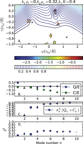
Figure 7. The same as figure 6 for the wave number  ,
,  ,
,  .
.
Download figure:
Standard image High-resolution image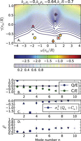
Figure 8. The same as figure 6 for the wave number  ,
,  ,
,  .
.
Download figure:
Standard image High-resolution imageWe now discuss several interesting trends that can be identified in this series of figures. We note that the trends identified are not universal—i.e., there is some minor variation to the observations described below. However, the main points are quite robust and the series of figures is representative of a broad range of wave numbers.
- (1)We first note that one NPEV corresponds quite closely to the unstable ITG mode, as expected from the pseudo-contours that are closely nested about the linear eigenvalue. This ITG mode is invariably the most energetic SVD structure. We also note that the NPEV for the ITG mode tends to drift away from its linear eigenvalue as the wavenumbers (kz and ky) increase, which is consistent with the increasingly vertically elongated pseudo-contours. As discussed above, this is a result of the two symmetry-breaking terms in the linear operator being, respectively, proportional to kz and ky.
- (2)As may be expected from the pseudospectra, a second NPEV closely corresponds to the marginally stable DW. Consistent with its linear counterpart, this mode has a relatively small Q and a smooth structure in velocity space, as evidenced by its small value of C/E. The DW linear eigenvalue is (aside from the ITG), the least stable eigenmode, which would suggest that it should achieve a penultimate degree of excitation in the nonlinear state. This is, surprisingly, often not the case, which brings us to perhaps the most puzzling element of the NPEV spectra.
- (3)As noted in section 4, the pseudo-spectra are extremely sparse in the lower region of the complex plane, providing little if any prediction of potential nonlinear structures that may be found here. Interestingly, a distinct NPEV with relatively high amplitude consistently appears in this region. This NPEV corresponds to the structure with, often, the second most (to only the ITG mode) energy in the spectrum. The mode has a similar frequency to that of the ITG mode and is strongly stable, often due to a substantially negative value of Q/E. This combination of relatively high amplitude and strong damping rate makes this mode a robust energy sink, as can be seen in the (C) panels. The properties of this mode evoke those of the MITG mode, which is identified in the collisionless linear eigenvalue spectrum but completely vanished when collisions are included (as they are in the nonlinear simulation). This begs the question whether the MITG mode, which is not an eigenmode of the underlying linear operator, reappears in the nonlinear turbulent fluctuations. This will be discussed in detail in the next section.
- (4)The remaining distinctive mode in the NPEV spectra is the fourth mode (diamond), which has a substantial value of C/E and appears consistently near
 . This, as with the remaining modes, cannot be clearly identified with any feature of the linear spectrum. These structures, which appear to be purely nonlinear creations, describe the small velocity space scales of the distribution function and collectively represent a non-negligible energy sink.

Having summarized the NPEVs, we redirect the readers attention to table (1), to which we can now add a final column denoting the modes identified in the nonlinear turbulent state.
5.3. The reappearance of MITG
As discussed above, a mode with properties very similar to those of the MITG mode appears in the NPEV spectra even though the MITG mode is completely absent from the underlying linear eigenvalue spectra. As it turns out, a closer examination of the pseudo-spectra serves to bridge the gulf between the pure linear and nonlinear analyses, resolving this apparent paradox. The key piece of information lies in the pseudo-eigenvectors defined by the right singular vectors described in relation to equation (16). These pseudo-eigenvectors represent the most resonant structures for the linear operator at a given point in the complex plane. As with linear eigenvectors or SVD vectors, various mode properties can be calculated from pseudo-eigenvectors. The contours of Q/E for the pseudo-eigenvectors are plotted throughout the complex plane in figure 9. The thick black contour separates regions of positive Q from negative Q. Interestingly, the region of strongly negative Q is found opposite (across the real axis) from the ITG eigenvalue in exactly the region where the MITG mode is found in the (collisionless) linear spectrum and its counterpart in the NPEV spectrum. Apparently, the MITG mode, which disappeared from the linear eigenvalue spectrum, remains 'just under the surface' in the pseudospectra, poised for excitation in the nonlinear turbulent state.

Figure 9. Contours of constant Q/E for pseudo-eigenvectors (solid black line denotes Q = 0) for the wave number  ,
,  ,
,  (corresponding to figure 6). Note the region of negative Q/E in the region opposite (across the real axis) from the ITG mode, demonstrating that the pseudo-eigenvectors retain the main property of the MITG mode even though the MITG mode is no longer an eigenvalue.
Download figure:
Standard image High-resolution imageThis identification of a remnant of the MITG mode in the pseudospectrum offers an explanation for the surprising reappearance of the mode in the nonlinear fluctuations—i.e., MITG-like structures represent some of the least-damped structures in the broad region of near-resonance with only very low-ε pseudospectral contours. However, the question remains as to why modes in this region of the complex plane are preferentially excited instead of, e.g., equally weakly damped structures with different frequencies. We propose here two factors that likely contribute to the preferential excitation of MITG modes.
First, the defining characteristic of the (M)ITG modes is the  cross-phase that determines the value of Q (i.e., the energy injected into the system by the instability). In the turbulent state, the nonlinearity will stochastically modulate this cross phase away from the value defined by the linear eigenmode, requiring, in combination with the positive-phase ITG mode, a negative-phase structure on which to project. The pseudospectra suggest that such a structure is most resonant in the MITG region of the complex plane.
Second, the dominant nonlinear coupling mechanism is likely to be strongest for resonant frequency triads that include a zonal (ky = 0) component (note that zonal coupling remains important in these simulations even though we do not remove the flux-surface-averaged potential in the equation for ϕ since this strongly suppresses the turbulence in slab simulations [20, 24]). This would entail three wave coupling between wave numbers  , where,
  ,
,  , and
, and  . The frequency of the zonal (ky = 0) component
  is (near) zero and the two finite ky wave numbers have frequencies with near-opposite signs so that
  . The reciprocal of this frequency sum is the correlation time of three wave interactions. In closure theories, the nonlinear transfer term is inversely proportional to this frequency sum so that couplings that satisfy this frequency cancellation would be strongly amplified (this has been studied in the context of stable mode coupling in related systems in [32, 39]). Such a coupling mechanism, in combination with the pseudospectral considerations discussed above, provide a compelling explanation for the reemergence of MITG in the nonlinear spectrum. Moreover, the frequency sum is seen to be descriptive of the nonlinear self-organization that favors the MITG and access to dissipation. As such, it could be useful as a proxy in nonlinear confinement optimization schemes like those pursued for stellarators [65].
5.4. Landau damping
The NPEV analysis also has something interesting to say about Landau damping. Figures 10 and 11 show the NPEV spectrum for high-kz wave numbers where the ITG and DW modes are stable due to Landau damping. The NPEVs follow the distortions in the pseudospectral contours and are clearly less damped than the linear eigenvalues that represent the Landau damping rates. This means that the Landau damping mechanism is much less effective than the pure linear solution would suggest. Figure 11 shows an NPEV that is a robust energy source even though there are no unstable linear eigenvalues. We generally observe that the nonlinear damping rate at high kz is strongly reduced (or even reversed) from the linear expectation. This suggests that the damping rates in critically balanced cascades [61–63] may be less than expected from linear Landau damping. This is consistent with recent work [26, 64] demonstrating that Landau damping rates are strongly modified by random sources intended to roughly represent a turbulent nonlinearity. This work suggests that pseudospectral or related non-modal techniques may prove useful in formulating advanced gyrofluid models that faithful reproduce Landau damping in a turbulent systems.

Figure 10. The same as figure 6 for a high kz wave number dominated by Landau damping:  ,
,  ,
,  . Note that the NPEVs follow the contours of the pseudospectra and are much more weakly damped than the linear damping rate.
Download figure:
Standard image High-resolution image
Figure 11. The same as figure 6 for a high kz wave number dominated by Landau damping:  ,
,  ,
,  . Note that the nonlinear structure is a robust energy source even though the corresponding linear growth rate suggests stability.
Download figure:
Standard image High-resolution image
6. Summary and discussion
Plasma turbulence often retains linear features in the nonlinear turbulent state. A growing body of work has used various decompositions to analyze plasma turbulence. In this paper we describe a new technique that combines the advantages (and mitigates the disadvantages) of linear eigenmode decompositions and SVD decompositions; using concepts motivated by pseudospectra, we associate a complex number, which we call the NPEV, with each structure extracted with SVD.
This technique is applied to a relatively simple gyrokinetic slab-ITG system, revealing novel features of the phase space structures. In the highly unstable region of the k-spectrum we observe the following features: (1) the highest-amplitude structure closely corresponds to the linear ITG mode, with the NPEV increasingly deviating from its corresponding eigenvalue as ky and kz increase. (2) A marginally stable DW identified in the linear spectrum also finds a close counterpart in the NPEV spectrum. (3) Surprisingly, we find a NPEV that closely corresponds to the MITG mode—a mode that has the same frequency but opposite growth rate as the ITG mode. The MITG mode is only an eigenvalue of the collisionless linear operator but not the collisional operator that underlies our nonlinear simulations. The pseudospectra serve to resolve this apparent paradox by revealing that the most-resonant vectors in the region of interest in the complex plane retain the features of the MITG mode even though there is no exact eigenvalue in this region. (4) Additional low-amplitude SVD structures have no apparent connection with the linear operator but collectively represent a non-negligible collisional dissipation mechanism.
The NPEVs also identify a consistent deviation of the nonlinear damping rates from the linear Landau damping rates for the high-kz regions of the spectrum. This is consistent with the corresponding pseudospectra, which are strongly distorted at high kz, making less damped regions of the complex plane surprisingly accessible. This observation may have implications for critically balanced cascades where energy is transferred through scale ranges expected to be robustly Landau damped. This paper suggests that non-modal techniques may be useful in formulating gyrofluid models that include accurate turbulent Landau damping rates.
We conclude that, as in other turbulent plasma systems, the scenario studied here can be characterized as strong wave turbulence—i.e. clear signatures of the linear mode properties persist within a strongly turbulent system. We add two additional insights to this picture—(1) there exist signatures of not only the most unstable mode, but also subdominant modes, and (2) some of these signatures are outside the realm of the eigenvalue approach and can only be understood through non-modal techniques like pseudospectra. In addition to refining our understanding of phase-space turbulence, this work may inform techniques (e.g., quaslinear treatments) for reduced modeling of turbulent transport. We also speculate that interesting insights may be obtained by applying similar techniques to neutral fluid turbulence, where SVD has been widely applied.
Acknowledgments
This research used resources of the National Energy Research Scientific Computing Center, a DOE Office of Science User Facility; and the Texas Advanced Computing Center (TACC) at The University of Texas at Austin. This work was supported by U S DOE Contract No. DE-FG02-04ER54742.