Experimental limits on the fidelity of adiabatic geometric phase gates in a single solid-state spin qubit

In the field of quantum information science, holonomic quantum computation [1–3] was proposed to take advantage of the geometric phase [4–6] which is believed to be impervious to certain types of errors. Geometric quantum logic gates were realized first with nuclear spins in liquid solutions of molecules using NMR techniques [7]. Geometric phase signal has also been observed with single superconducting qubits [8] and trapped ions [9].

While it is often thought that geometric phase is less sensitive to fluctuations in the control fields, it was realized that a very general feature of such adiabatic Hamiltonians is the unavoidable decay of the quantum state caused by control field fluctuations [10]. The fundamental reason for this decay is that the geometric phase is always accompanied by the dynamic phase in non-degenerate quantum systems. Dynamical decoupling techniques such as spin echo and XY sequences can cancel the average dynamic phase caused by the control field, and filter out environmental noise that remains correlated within the clock time τ between the decoupling pulses within the sequence [11–13]. But the sequences are still sensitive to the second moment in the fluctuations of the dynamic phase caused by the control fields at frequencies which are on the order of, or higher than, the clock frequency. The real question then is how much protection do adiabatic geometric quantum logic gates have from such control field noise.

Nitrogen-vacancy (NV) centers in diamond are among the most promising candidates for quantum information applications, highly sensitive nanoscale quantum sensors, biological markers, and as single photon emitters in quantum communication[14]. Such solid-state single spin qubit is ideal for exploring geometric phase and the fidelity of geometric logic gates because of the remarkable degree of coherent control achievable with modern technology [15]. Proposals to measure Berry phase in mechanically rotating diamond crystal [16], and for application in gyroscopes [17, 18] also motivate our experiments.

In this work, we report our measurement of the Berry phase, and the fidelity of adiabatic single qubit geometric phase gates, in the system of a single NV center in diamond. We apply a carefully tailored time-dependent adiabatic Hamiltonian, via rotating frame off-resonant microwave driving waveforms; as well as a resonant spin echo interferometry sequence to filter out environmental noise, and cancel the accompanying average dynamic phase from the time-dependent Hamiltonian. We have studied through careful experiments and numerical calculations, the systematic deviations in the geometric phase caused by imperfect driving waveforms, as well as the decay of the fidelity in the phase gate from various noise sources. We conclude that the fidelity is ultimately limited by dynamical phase contributions occuring due to the naturally present control field noise.

Our work is the first to experimentally measure the decay of the gate fidelity of an adiabatic geometric phase gate in the complex solid-state environment that is created by the interaction of a single solid-state electronic spin qubit with the slowly varying nuclear spin bath in diamond. Theoretical work in adiabatic and non-adiabatic quantum control settings [10, 19, 20], and in other solid-state qubits such as quantum dots [21, 22] and superconducting qubits [23, 24] has found that geometric phase can be affected by the environment and control field noise. At the end of our paper, we also speculate on what our results could potentially mean for geometric quantum information processing with solid-state qubits.

In quantum mechanics, the Hamiltonian for a spin-$\tfrac{1}{2}$ qubit interacting with an external magnetic field is given by $H={\hslash }{\gamma }_{s}{\bf{B}}\cdot {\boldsymbol{\sigma }}/2$, where ${\boldsymbol{\sigma }}=({\sigma }_{x},{\sigma }_{y},{\sigma }_{z})$ are the Pauli operators, ℏ is Planck's constant, ${\gamma }_{s}$ is the appropriate gyromagnetic ratio for the particle, and $| {\bf{B}}|$ is the magnetic field vector. When the external magnetic field varies adiabatically, the spin vector precesses around the external field ${\bf{B}}$, and acquires a dynamic phase ${\beta }_{d}={\gamma }_{e}{Bt}$ where $B=| {\bf{B}}|$, which depends on the closed path. In addition, Berry showed that the spin acquires an additional phase ${\beta }_{g}$ that is independent of the nature of the path and depends purely on the geometry [4] as shown in figure 1(a). In the Bloch sphere picture (figure 1(b)), as the field ${\bf{B}}(t)$ traces out a cone with angle θ, the spin vector ${\bf{S}}(t)$ remains perpendicular to ${\bf{B}}$. When ${\bf{B}}$ completes a closed circuit which traces out the solid angle Θ, the spin vector has acquired an additional geometric phase ${\beta }_{g}={\rm{\Theta }}$. In classical dynamics, an analog to this phenomenon is the Hannay angle, which can be illustrated by the rotation angle acquired by a rigid disc spinning around an axle that adiabatically traces out a closed contour [25].

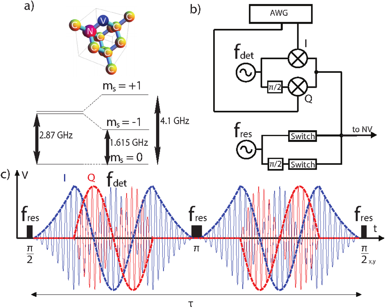
Zoom In Zoom Out Reset image size

The NV center (figure 2(a)) is a spin-1 system in the ground state, quantized along the ${{\rm{C}}}_{3v}$ symmetry axis between the nitrogen and vacancy sites, with the $| {m}_{s}=0\rangle$ and $| {m}_{s}=\pm 1\rangle$ levels split by 2.87 GHz at zero magnetic field. The spin state can be initialized by optical pumping with 532 nm laser excitation, and the spin polarization can be detected by measuring the spin-dependent fluorescence signal. We use a single NV center in a type-IIa bulk diamond sample, and apply a static magnetic field B₀ oriented along the NV centers z-axis, allowing us to form a pseudo-spin-1/2 qubit system with the $| {m}_{s}=0\rangle \leftrightarrow | {m}_{s}=-1\rangle$ spin states. The magnetic field is chosen to bias the system near the excited-state level anti-crossing, resulting in complete polarization of the associated ${}^{14}{\rm{N}}$ nuclear spin of the NV center [26] and realizing a nearly ideal two-level system for our experiments. Microwave pulses are applied to the NV center using an impedance-matched microstrip line coupled to a thin copper wire on the diamond surface, allowing us to attain a $\pi /2$ rotation in ∼20 ns.

Zoom In Zoom Out Reset image size

In the rotating frame of the microwave drive, and under the rotating wave approximation, the Hamiltonian for the NV center can be written as

$$\begin{eqnarray}&&H={\hslash }{\rm{\Delta }}{\sigma }_{z}+{\hslash }{\rm{\Omega }}({\sigma }_{x}\mathrm{cos}{\rm{\Phi }}+{\sigma }_{y}\mathrm{sin}{\rm{\Phi }}).\end{eqnarray} \tag{ 1 }$$

Here Δ is the detuning between the microwave and the transition frequency, Ω is the Rabi frequency of the drive field and Φ is an adjustable control phase of the microwave. In the rotating frame, we can immediately identify the effective magnetic field as given by ${\bf{B}}=({\rm{\Omega }}\mathrm{cos}{\rm{\Phi }},{\rm{\Omega }}\mathrm{sin}{\rm{\Phi }},{\rm{\Delta }})$. In our experiments, we typically keep Δ fixed and trace circular paths with different radii Ω. The cone angle in our experiment would therefore by given by $\mathrm{cos}\theta ={\rm{\Delta }}/{({{\rm{\Omega }}}^{2}+{{\rm{\Delta }}}^{2})}^{1/2}$.

The corresponding adiabatic circuit for the magnetic field can be achieved by fast amplitude and phase modulation of the applied microwave drive field [7, 8], using an IQ modulator and arbitrary waveform generator (AWG), as shown in figure 2(b). We measure Berry's phase using a spin echo interference experiment. We apply two types of microwaves to the system as shown in figure 2(c): one at a frequency f_det that carries out the adiabatic circuit for ${\bf{B}}$, and another tuned to the resonance transition frequency f_res that is used for the spin echo interference, and subsequent state tomography to extract the spin vector. The spin echo sequence initializes the qubit into an eigen-state of ${\sigma }_{x}$ with a resonant $\pi /2$ pulse. The effective field ${\bf{B}}$ created by the off-resonant drive traces out a contour C in figure 1(a), and the direction is set by the phase modulation Φ. The relative quantum phase between the states $| 0\rangle$ and $| 1\rangle$ during the adiabatic circuit is given by ${\phi }_{\pm }=({\beta }_{d}\mp {\beta }_{g})$ where ± denotes counter-clockwise (clockwise) direction. Due to the resonant π-pulse in the spin echo sequence, the cumulative relative phase becomes $\phi ={\phi }_{-}-{\phi }_{+}=2{\beta }_{g}$, and increasing the number of times (N) that we trace the contour gives us ${\beta }_{g}=(N/2){{\rm{\Theta }}}_{C}$. The resonant π-pulse also cancels any fluctuations in environmental or other fields that occur on timescales slower than the echo sequence, thereby extending the decoherence time from the Ramsey dephasing time ${T}_{2}^{*}$ to T₂.

At the end of the sequence, we can extract the values of the spin vector through quantum state tomography. The value of $\langle {S}_{z}\rangle$ can be obtained using either Rabi oscillations or rapid adiabatic passage experiment to calibrate our fluorescence levels (see appendices D and E). The $\langle {S}_{x}\rangle$ and $\langle {S}_{y}\rangle$ values can be obtained by applying a $\pi /2$ pulse around the different axes x or y, serving as a tomography pulse. The experimental phase can then be extracted as $\phi =\mathrm{arctan}(\langle {S}_{y}\rangle /\langle {S}_{x}\rangle )$. Even in the presence of decoherence, which is a minor effect in our experiments, the coherence in either x or y direction would be equally affected and thereby will not alter the geometric phase we measure from taking the ratio. The total pulse sequence time and the shape of the waveforms was chosen to both preserve adiabaticity and to allow for the local spin environment of our qubit to return to its original state. (See appendix E.)

The data in figure 3(a) shows the values of $\langle {S}_{x}\rangle$ and $\langle {S}_{y}\rangle$ measurements as the Rabi frequency Ω was varied while the detuning Δ remains fixed. The expected signal here from theory is

$$\begin{eqnarray}\langle {S}_{x}\rangle & = & A\mathrm{cos}(N{\rm{\Theta }}),\\ \langle {S}_{y}\rangle & = & -A\mathrm{sin}(N{\rm{\Theta }}),\\ {\rm{\Theta }}={\rm{\Theta }}({\rm{\Omega }}) & = & 2\pi \left(1-\displaystyle \frac{{\rm{\Delta }}}{{({{\rm{\Omega }}}^{2}+{{\rm{\Delta }}}^{2})}^{1/2}}\right)\end{eqnarray} \tag{ 2 }$$

as shown in figure 3 (a) dashed lines. To verify that the data observed is really due to geometric phase and not other artifacts, we carried out measurement where we do not reverse the direction of the contour in second half of sequence. We observed no oscillations since both dynamic and geometric phase are canceled. This result is shown in appendix H, and also replotted in figure 3(c) as the N = 0 data.

Zoom In Zoom Out Reset image size

We can use the Berry phase for quantum logic by carrying out a single qubit geometric phase gate $U(\phi )=\left(\begin{array}{ll}1 & 0\\ 0 & {{\rm{e}}}^{{\rm{i}}\phi }\end{array}\right)$. For instance, if ${{\rm{\Theta }}}_{C}=\pi /4$, then for N = 2, we obtain a $\pi /2$ phase gate. The gate fidelity F_U is obtained by averaging the state fidelity ${F}_{j}=\langle {\psi }_{j}| U{\rho }_{\mathrm{exp}}{U}^{\dagger }| {\psi }_{j}\rangle$ for the 6 input states $| {\psi }_{j}\rangle =\pm | X\rangle ,\pm | Y\rangle ,\pm | Z\rangle$ [27]. Our state tomography measurements of $\langle {S}_{x}\rangle$ and $\langle {S}_{y}\rangle$ in figure 3(a) allow us to calculate the state fidelity for $| {\psi }_{j}\rangle =\pm | X\rangle ,\pm | Y\rangle$ as ${F}_{\pm X,\pm Y}=(1+\langle C\rangle )/2=0.979\pm 0.022$, where $\langle C\rangle =\sqrt{{\langle {S}_{x}\rangle }^{2}+{\langle {S}_{y}\rangle }^{2}}$ is the spin coherence. Combined with our measurements in appendix E, we obtain the state fidelity for $| {\psi }_{j}\rangle =\pm | Z\rangle$ to be ${F}_{\pm Z}=0.976\pm 0.035$, and therefore the gate fidelity to be ${F}_{U}=0.978\pm 0.026$. In our numerical simulations below (section 4), we show that this gate fidelity is primarily limited by the dynamical phase contribution to the adiabatic geometric gate.

The theoretical prediction shown in figure 3(a) differs from the measured values in a systematic fashion. The experimental data oscillates faster than theory, meaning the measured phase is larger than theoretical prediction with our microwave parameters. We should also note that a similar deviation from theory can be seen in another solid-state qubit system, although it was not explicitly investigated in that work [8]. The systematic deviation is not simply due to incorrect calibration of our microwave drive amplitude or other parameters. In figure 3(c) we have extracted the quantum phase ϕ for different values of N from our experiments (markers), and compared it to the analytical expressions in equation (2) (dashed lines). The data in figure 3(c) does not scale linearly with the solid angle, as would be expected from Berry's result, but instead shows clear nonlinearity with increasing solid angle. Shifts of the Berry phase due to non-closed paths in parameter space caused by environmental or control field noise are expected, but the magnitude of the shifts are typically quite small [22]. We note that the discrepancy does not change our conclusion above on the fidelity of the geometric quantum phase gate, as we merely have to recalibrate the solid angle ${{\rm{\Theta }}}_{C}$ required to carry out the $\pi /2$ geometric phase gate.

To search for an explanation of this discrepancy, a series of test experiments were carried out including power calibration test, fluorescence levels test, adiabaticity test and test of single channel nonlinearity of IQ modulator. We have verified that the microwave power is correctly calibrated, the fluorescence level used for qubit measurement is correctly calibrated, and the adiabaticity parameter is kept small (see appendices C–E) in our experiments. However, in the test of single channel nonlinearity of IQ modulator, we noticed a misalignment between the experimental data and theory (see appendix F). Figure 4(a) shows the distortion of the modulating waveform caused by the single channel nonlinearity. The corresponding circuit traced out by the hamiltonian is shown in figure 4(b). The distortion of the contour results in changing the solid angle ${\rm{\Theta }}\to {{\rm{\Theta }}}_{\mathrm{exp}}$.

Zoom In Zoom Out Reset image size

An additional source for distortion is amplitude imbalance in I and Q channel. If we input the same DC voltage to I or Q channel, the output microwave amplitude may be different because of IQ imbalance. When we measure the output microwave amplitude, a microwave mixer is used to step down the frequency of microwave into the bandwidth of our oscilloscope, and the amplitude of microwave is measured with the oscilloscope. We estimated the amplitude imbalance to be $\epsilon \sim 10\%$, same as the accuracy of our measurement.

We performed numerical simulation of our Berry phase experiment for comparison with our experimental data. The microwave sequence is separated into small time steps $(\delta t\ll \tfrac{1}{{\rm{\Omega }}},\tfrac{1}{{\rm{\Delta }}})$, and the time-dependent Hamiltonian in the rotating frame is approximately constant during each time step. The quantum state will evolve as:

$$\begin{eqnarray}&&| {\rm{\Psi }}(t+\delta t)\rangle =\mathrm{exp}\left(-{\rm{i}}\displaystyle \frac{\hat{H}(t)}{\bar{h}}\delta t\right)| {\rm{\Psi }}(t)\rangle .\end{eqnarray} \tag{ 3 }$$

Any imperfections in our microwave drive field can be easily taken into account by modifying the Hamiltonian $\hat{H}(t)$. Here we took both single channel nonlinearity and amplitude imbalance of the IQ modulator into account. The on-resonance microwave pulses for spin echo are assumed perfect, and decoherence is not taken into account because the sequence time $\tau \ll {T}_{2}$. The complete Hamiltonian used in our simulation is:

$$\begin{eqnarray}\hat{H}(t) & = & {\rm{\Delta }}\hat{{S}_{z}}+{\rm{\Omega }}\overset{\mathrm{single}\ \mathrm{channel}\ \mathrm{nonlinearity}}{\overbrace{({aI}(t)+{bI}{(t)}^{3})}}\hat{{S}_{x}}\\ & & -{\rm{\Omega }}\overset{\mathrm{single}\ \mathrm{channel}\ \mathrm{nonlinearity}}{\overbrace{(a(\underset{\mathrm{IQ}\ \mathrm{imbalance}}{\underbrace{(1+\epsilon )}}Q(t))+b{(\underset{\mathrm{IQ}\mathrm{imbalance}}{\underbrace{(1+\epsilon )}}Q(t))}^{3})}}\hat{{S}_{y}},\end{eqnarray} \tag{ 4 }$$

where a and b are extracted from our measurement of single channel nonlinearity (see appendix F).

In figure 3(b), the results of the numerical simulation for Berry Phase experiments are shown, using the Hamiltonian from equation (4); with parameters a, b, measured from experiments (see appendix F). In figure 3(c) we have extracted the quantum phase ϕ for different values of N from both experiments and simulations. As seen in both these figures, the experimental results more closely match our numerical simulations rather than the simple analytical expressions of equation (2). Although the agreement is not perfect, the nonlinear scaling with increasing solid angle is evident in our simulation results.

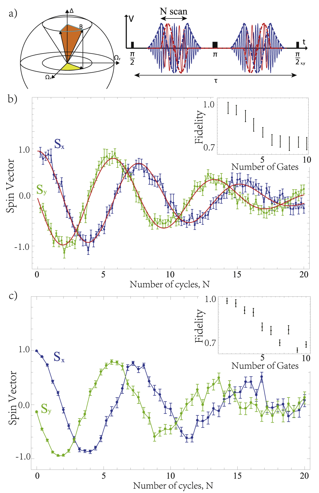
Our final set of measurements explores the question of how the geometric phase decays. Decay of the geometric phase is an important parameter to be measured for feasibility of geometric quantum information processing [1, 2] and for NV spin gyroscopes and mechanical rotation sensors [16–18]. As shown in figure 3(a), we were unable to detect any obvious geometric dephasing over the solid angles obtainable by scanning the Rabi frequency Ω. To increase the amount of geometric phase accumulated, we used the fact that the total quantum phase $\phi =N{{\rm{\Theta }}}_{C}$. Hence, we carried out an experiment with N (number of cycles the spin traces out) continuously varying while keeping the solid angle ${{\rm{\Theta }}}_{C}$ fixed, using the pulse sequence in figure 5(a).

Zoom In Zoom Out Reset image size

Our experimental data in figure 5(b) clearly showed decay as the amount of geometric phase is increased. The inset to figure 5(b) depicts the measured gate fidelity F_U for multiple operations of the $\pi /2$ phase-shift gate $U(\phi =\pi /2)$. Note that the signal decays and the gate fidelity rapidly approaches the classical limit ${F}_{c}=2/3$ for a single qubit gate [28] after ∼10 repetitions. We also compare our results to the numerical simulation in figure 5(c), which is explained in more detail below. Our conclusion from the simulation is that both the decay in the geometric phase, and the decay in the fidelity, are well explained by the dynamical phase fluctuations caused by control field noise.

Before discussing the numerical simulation results, we examine the potential theoretical sources for decay of the geometric phase ${\beta }_{g}=(N/2){{\rm{\Theta }}}_{C}$. The decay could be potentially assigned into two major sources

• (1)  
  Geometric dephasing due to slow fluctuation in Δ.
• (2)  
  Geometric dephasing due to slow fluctuation in Ω

here the word 'slow' means frequencies lower than the clock frequency of the spin echo. Indeed this was the model used in [8] to study geometric dephasing. We can estimate the strength of these fluctuations for Δ and Ω independently for our NV center from Ramsey and Rabi measurements. Assuming a gaussian model for the noise spectrum in Δ, we obtain the following expression for the decay in the Berry phase as a function of the circuital number N:

$$\begin{eqnarray}&&\langle {S}_{x}\rangle =A\mathrm{cos}(N{{\rm{\Theta }}}_{C})\mathrm{exp}(-{(N/{N}^{*})}^{2}),\end{eqnarray} \tag{ 5 }$$

where

$$\begin{eqnarray}&&{N}^{*}=\displaystyle \frac{\sqrt{2}}{\alpha {\sigma }_{{\rm{\Delta }}}}=\displaystyle \frac{2\pi {T}_{2}^{*}}{\alpha }\end{eqnarray} \tag{ 6 }$$

${\sigma }_{{\rm{\Delta }}}$ is the standard deviation of the noise, $\alpha =| \partial {{\rm{\Theta }}}_{C}/\partial {\rm{\Delta }}| =\tfrac{{{\rm{\Omega }}}^{2}}{{({{\rm{\Omega }}}^{2}+{{\rm{\Delta }}}^{2})}^{3/2}}$ . Given the numerical values for these parameters in our experiments, we obtain a prediction of ${N}^{*}\sim 400$, which is well above the actual value ${N}^{*}\sim 14$ from the fits shown in figure 5(b). Therefore, we eliminate the slow noise in Δ from this environment as a main source of the decay in our data.

The slow noise in Ω can be independently measured with a long-time on-resonance Rabi experiment. From this we get ${\sigma }_{{\rm{\Omega }}}\lt {\sigma }_{{\rm{\Delta }}}$(see appendix G). This implies that the slow noise in Ω contributes even less than in Δ. Because the Berry phase depends only on Δ and Ω, and neither fluctuation in Δ nor in Ω is sufficient to explain such a large decay, we concluded that this decay of signal is not due to geometric dephasing.

We note here that slow noise in Δ dominates as the geometric dephasing in superconducting qubit systems, as shown in [8]. Previous experimental work in superconducting qubits was restricted to studying symmetric, artificially induced control noise on geometric phase, and measuring only the decay of the quantum phase [29, 30]. Our experiments are conducted in a different regime, where the noise is asymmetric, intrinsic to the signal generators, and we explicitly examine the effect of the control noise on the fidelity decay of the geometric quantum phase gate.

We attribute the decay to fluctuations in dynamic phase. This effect has been predicted in [10], but has not previously been measured with single spin qubit systems. The average dynamic phase accumulated during each half of the sequence is:

$$\begin{eqnarray}&&{\beta }_{d}=\sqrt{{{\rm{\Omega }}}^{2}+{{\rm{\Delta }}}^{2}}\times \displaystyle \frac{\tau }{2},\end{eqnarray} \tag{ 7 }$$

where τ is the spin echo sequence time. As previously explained, in our experiments, the measured phase is $\phi ={\phi }_{-}-{\phi }_{+}=2{\beta }_{g}$ where the dynamic phase ${\beta }_{d}$ in ${\phi }_{-}$ and ${\phi }_{+}$ cancels each other. However, fast fluctuations (fluctuations occurring within the sequence time) in ${\beta }_{d}$ cannot be canceled. Such fluctuations in dynamic phase will result in fluctuation in our measured phase ϕ, causing dephasing. So the reason for the decay of signal could be

• (1)  
  Dynamic dephasing due to fast fluctuation in Δ.
• (2)  
  Dynamic dephasing due to fast fluctuation in Ω.

Fast fluctuations in Δ, from the environment field itself, should also result in decay when no external microwave field is present, i.e. spin echo decay which is characterized by T₂. The value of ${T}_{2}\sim 300\;\mu {\rm{s}}$ we measured is significantly larger than the decay time observed here. We cannot completely eliminate fast frequency fluctuations in the microwave synthesizer or in the AWG, but we know that we can use either synthesizer to perform the spin echo measurements with similar results, implying that the phase noise of the synthesizers could not result in this decay. We therefore conclude that fast fluctuations in Ω are most likely the important cause of dynamic dephasing.

We set a simplified model for our numerical simulation: the microwave amplitude has a random Gaussian fluctuation (${\sigma }_{{\rm{\Omega }}}$) from the first half of spin echo to the second half. With this simplified model, the results of our simulation with all other parameters taken from the experiment are shown in figure 5(c), and show good consistency with our experimental data. The inset to figure 5(c) shows the calculated gate fidelity F_U for our numerical simulation, and also agrees well with our experimentally measured gate fidelity. The fast fluctuation ${\sigma }_{{\rm{\Omega }}}/{\rm{\Omega }}$ used in simulation is 8 × 10⁻³, close to the bit resolution of our AWG (∼2 × 10⁻³, 10 bit from −1 to 1), and is consistent with decay observed in our long time Rabi data (see appendix G). Finally, in our numerical simulations, we have assumed perfect state preparation, no decoherence, and no readout noise. The only deviation from the ideal case is the control field noise, and the results of the simulation shown in figure 5(c) agrees well with the data of figure 5(b). In particular, note that the gate fidelity for 1 gate operation from experimental data in figure 5(b) is 0.978 ± 0.040, and the gate fidelity for 1 gate operation in our numerical simulation in figure 5(c) is 0.973 ± 0.017.

We also performed experiments to measure dynamic dephasing without Berry phase involved, to further verify our claim that the decay is due to dynamic phase fluctuation. As shown in the inset to figure 6 (a), we used similar microwave sequence as our experiments to measure geometric dephasing (figure 5(a)). However, instead of letting the effective drive field trace a contour in parameter space, here the drive field remains in the same direction during the time t. We observed the decay in our measured signal shown in figure 6(a). This decay must be due to dynamic dephasing, because no geometric phase is involved at all. In figure 6(b), we carried out the numerical simulations for the experiments in figure 6(a) and obtain good agreement with the data. Just as importantly, this decay in dynamic phase signal matches the time scale of our Berry phase decay data.

Zoom In Zoom Out Reset image size

Experiments probing the effect of noise on geometric phase and geometric quantum logic gates are surprisingly few and far between. Our work reports on detailed measurements of the adiabatic geometric phase in a single solid-state spin qubit, and on the effects of noise and control field imperfections on the geometric phase signal as well as the fidelity of geometric phase gate. We have found that the spin echo sequence cancels the average dynamic phase imparted by control field as well as slow dynamic phase fluctuations from the environment, but it cannot cancel the second-order moment of the control noise that occurs faster than the spin echo clock frequency. Our experimental results and numerical simulation show that the decay in the fidelity of the phase gate is due to these fluctuations. In general, we expect that any adiabatic geometric quantum logic gate operation that relies on cancellation of the dynamic phase will have to account for such control field fluctuations, which agrees also with the conclusions of [10].

One possible direction for future work is to probe the spectrum of fast fluctuations. While our frequency is sufficiently high that $1/f$ noise in the electronics should become small, we could potentially use our highly sensitive measurement to map out the spectral dependence of the noise by changing the spin echo clock frequency. Another direction is to start with signal generators that have much lower levels of amplitude noise (higher vertical bit resolution), and add in specially tailored noise to examine the effects on the geometric quantum logic gate fidelity. We can then compare the measured values using our numerical simulations, which seem to be in good agreement with our experimental results reported here.

Fundamentally, the problem is that the adiabaticity condition imposes an upper limit to the rate with which the Hamiltonian can be modulated for non-degenerate quantum systems, and this makes the experiment sensitive to fluctuations in dynamical phase that occur faster than the modulation rate. An obvious question would be to ask what happens when non-adiabatic, non-Abelian geometric phases in degenerate quantum systems are used instead, as proposed for instance in [3]. Typically, the states themselves are not perfectly degenerate but are instead shifted close to degeneracy using a pair of driving fields tuned to the transitions with a third level, for instance in a V or Λ-level configuration. Reference [31] has studied theoretically the effect of control field fluctuations on non-adiabatic geometric quantum logic operations and found that such fluctuations can be mitigated under specially tuned circumstances but in general do play an important role. Recently, [32] demonstrated non-adiabatic non-Abelian geometric gates with superconducting qubits. In their work, they concluded that the decrease in fidelity reported is partially due to dynamic phase fluctuations, similar to our results with Berry phase. We expect that our results and extensions of our work could also be important in understanding recent experimental results for non-adiabatic geometric gates with NV centers [33] and all-optical geometrical phase manipulation with NV centers [34].

This work was supported by the DOE Office of Basic Energy Sciences (DE-SC 0006638) for development of geometric quantum control techniques, key equipment, materials and effort. GD gratefully acknowledges support from the Alfred P Sloan Foundation.

NV centers in our type-IIa single crystal diamond sample (sumitomo with [1 1 1] orientation) are located with our home-built confocal microscope. A high NA dry microscope objective (Olympus 0.95 NA) is used in this confocal setup for NV excitation and collection of fluorescence emission. Phonon-mediated fluorescent emission (650–750 nm) for the single NV center is detected under coherent optical excitation (LASERGLOW IIIB 532 nm laser) using a single photon counting module(PerkinElmer SPCM-AQR-14-FC). Green excitation of the NV center polarizes the electron spin into $| {m}_{S}=0\rangle$ sublevel of the ³A₂ ground state due to optical pumping. The rate of fluorescence signal counts varies for the $| {m}_{S}=0\rangle$ and $| {m}_{S}=\pm 1\rangle$ states, which enables the optical detection of the electron spin. The photon counting takes place at the both ends of the optical excitation pulse (figure A1(b)). The counts at the beginning known as 'signal' (S_i) is highly dependant on the NV state while the counts at the end of optical excitation known as 'reference' (R_i) is not. By taking the ratio of S_i and R_i as our fluorescence level (a.u.), we minimize the effect of laser fluctuations on our experiments. A DC bias magnetic field ${B}_{0}\approx 450$ Gauss is applied along the NV axis by a permanent magnet. The transition frequency between $| {m}_{S}=0\rangle$ and $| {m}_{S}=-1\rangle$ states is measured by optically detected magnetic resonance (ODMR) experiment and pulsed ESR frequency scan experiment (figure A1 (a)). Detuned microwave for Berry phase experiment is generated by Rohde and Schwarz (SMIQ03B) signal generator with built-in IQ modulator. On resonance microwave is generated by PTS3200 synthesizer. Both microwaves are delivered via a 20 μm diameter copper wire placed on the diamond sample. The input waveforms for IQ channels are generated by Tektronics AWG520 AWG (1G sample/s). The value of Δ is extremely well controlled in our experiments as we frequently track the resonance frequency of the NV center. Both synthesizers in our experiment are synchronized by an atomic clock and measured to drift less than $\sim 1\times {10}^{-3}\;\mathrm{Hz}$, and this is tested by mixing the two microwaves from the two synthesizers under the same command frequency with a mixer and measuring the DC output of the mixer.

Zoom In Zoom Out Reset image size

The ${}^{13}{\rm{C}}$ nuclear spin bath that has a natural abundance of $\approx 1.1\%$ effectively produces a random field with frequency set by the nuclear gyromagnetic ratio ${\gamma }_{n}=2\pi (10.75)$ MHz T⁻¹ and the DC bias field B₀. This random field causes collapses and revivals in the CP signals, as shown in figure B1. For Berry phase experiment, it is required to operate on a revival point of spin echo sequence. In our Berry phase amplitude scan, the spin echo sequence time is set to the first revival. In N scan, the sequence time is set to the fifth revival.

Zoom In Zoom Out Reset image size

To test the frequency response of our microwave power, Rabi oscillation were measured under detuned microwave driving field with different detuning frequencies. As microwave detuning increases, observed Rabi oscillation frequency will increase as:

$$\begin{eqnarray}&&{\rm{\Omega }}({\rm{\Delta }})=\sqrt{{\rm{\Omega }}{(0)}^{2}+{{\rm{\Delta }}}^{2}}\end{eqnarray} \tag{ 8 }$$

oscillation amplitude will decrease as:

$$\begin{eqnarray}&&\mathrm{amp}({\rm{\Delta }})=\mathrm{amp}(0)\displaystyle \frac{{\rm{\Omega }}{(0)}^{2}}{{\rm{\Omega }}{(0)}^{2}+{{\rm{\Delta }}}^{2}}\end{eqnarray} \tag{ 9 }$$

and the equilibrium position of oscillation will increase as:

$$\begin{eqnarray}&&{bkg}({\rm{\Delta }})={bkg}(0)+\mathrm{amp}(0)\displaystyle \frac{{{\rm{\Delta }}}^{2}}{{\rm{\Omega }}{(0)}^{2}+{{\rm{\Delta }}}^{2}}.\end{eqnarray} \tag{ 10 }$$

This measurement of Rabi oscillations are taken with synthesizer for detuned microwave and through IQ modulator show in figure 2(b). The data (figure C1) shows no evidence of mis-calibration of our Rabi frequency Ω in detuned microwave.

Zoom In Zoom Out Reset image size

In our experiments, the direct signal we were measuring is fluorescence counts. The fluorescence counts signal was mapped to probability in $| 0\rangle$ or $| 1\rangle$ state by calibration of fluorescence levels at $| 0\rangle$ and $| 1\rangle$ states with Rabi oscillation. However, imperfections in π pulses might result in imperfect rotations and thereby cause errors in the fluorescence calibration.

Adiabatic passage is another way of calibrating fluorescence levels, and is used to check our Rabi oscillation calibration. By modulating both the amplitude and frequency of the driving microwave, an effective magnetic field adiabatically varying from $+z$ direction to $-z$ direction was created, as shown in figure D1(a). The detuned microwave starts ramping up at $t={t}_{0}$ while modulating its frequency, and then ramps back down to 0 with an opposite detuning at $t={t}_{f}$. The magnitude of the effective B field is 12.5 MHz. Fluorescence level at different time t was measured and shown in figure D1(b).

Zoom In Zoom Out Reset image size

The data points before t₀ and after t_f is fitted to fluorescence levels in $| 0\rangle$ and $| 1\rangle$ state resplectively. The fitted fluorescence levels fall in the confidence interval from our Rabi calibration, meaning our fluorescence level calibration is accurate.

The Berry phase theory is based on adiabatic approximation. The Berry phase is not robust to transitions between $| 0\rangle$ and $| 1\rangle$ state, and there could be a discrepancy from the theory if the transition probability is not negligible.

In order to check our adiabaticity, almost the same waveform as Berry phase experiment (N = 2) was used. The only difference is that the first $\pi /2$ pulse and the last $\pi /2$ pulse were removed figure E1. If the adiabatic condition is good, the spin should stay in $| 0\rangle$ state before the π pulse and stay in $| 1\rangle$ state after the π pulse. The probability in state $| 0\rangle$ at the end of the sequence should be close to 0. This probability in state $| 0\rangle$ for both scanning ramping up/down time T_a and the scanning cyclic period T is shown in figure E1.

Zoom In Zoom Out Reset image size

The data is taken at 5 MHz detuning, 12.5 MHz Rabi frequency. Adiabaticity parameter (shown as red curves) was calculated according to T(T_a) using equations:

$$\begin{eqnarray}A & =\displaystyle \frac{\tfrac{2\pi }{T}\mathrm{sin}\theta }{2\sqrt{{{\rm{\Delta }}}^{2}+{{\rm{\Omega }}}^{2}}} & (\mathrm{for}\ \mathrm{cyclic}\ \mathrm{motion}),\\ A & =\displaystyle \frac{1}{2{\rm{\Delta }}{T}_{a}}\sqrt{\displaystyle \frac{{{\rm{\Omega }}}^{2}}{{{\rm{\Delta }}}^{2}+{{\rm{\Omega }}}^{2}}} & (\mathrm{for}\ \mathrm{ramping}).\end{eqnarray} \tag{ 11 }$$

In our Berry phase experiments (10 MHz detuning, 12.5 MHz Rabi frequency for amplitude scan), we chose $T\geqslant 800\;\mathrm{ns}$, ${T}_{a}\geqslant 350\;\mathrm{ns}$. (See table E1 for details.) We believe we were well within the adiabatic regime.

Table E1.  Time parameters used in Berry phase experiments.

Parameter	Experiment	Value
Period of cycle T	Ω scan N = 2	$1\;\mu {\rm{s}}$
	Ω scan N = 3	$0.8\;\mu {\rm{s}}$
	N scan	$0.8\;\mu {\rm{s}}$
Ramp time Ta	Ω scan N = 2	$0.45\;\mu {\rm{s}}$
	Ω scan N = 3	$0.35\;\mu {\rm{s}}$
	N scan	$0.45\;\mu {\rm{s}}$
Spin echo sequence time τ	Ω scan N = 2	$4\;\mu {\rm{s}}$
	Ω scan N = 3	$4\;\mu {\rm{s}}$
	N scan	$20\;\mu {\rm{s}}$

The single channel nonlinearity test is based on Rabi oscillation measurement. In Rabi experiment, we sent the microwave through IQ modulator, and we can change the DC voltage input for I channel, while Q channel input stays at 0. The measured signal is:

$$\begin{eqnarray}&&S=\mathrm{cos}({V}_{i}{\rm{\Omega }}t).\end{eqnarray} \tag{ 12 }$$

Here V_i is normalized DC input for I channel, and Ω is the Rabi frequency when V_i reaches 1. To test single channel linearity, the microwave pulse length t is fixed to 100 ns, we measured the signal at different V_i. As shown in figure F1(a), a clear discrepancy between data and expected values (green curve) was found. The data is fitted to nonlinear function ${{aV}}_{i}+{{bV}}_{i}^{3}$ instead. The fit parameters are $a=1.17,b=-0.17$.

Zoom In Zoom Out Reset image size

Noticing figure F1(a) inset, because of this nonlinearity, the actual value of V_i is slightly larger than the command value. As a result, the actual trajectory in parameter space the spin will trace out is distorted (figure F1(b)). The actual trajectory spans a larger solid angle, which coincides our Berry phase data. The single channel nonlinearity of the IQ modulator could be an important reason of our Berry phase data discrepancy.

A simple long time Rabi experiment was done to test the microwave power stability. If the microwave amplitude has a probability distribution around the expected value, the Rabi signal will decay as pulse length increases, which is shown in figure G1. The data is taken at the same microwave power as the Berry phase experiment (12.5 MHz), and the total experiment time is comparable to Berry phase experiment. From the fit parameter we get the time scale of decay ${T}_{1}^{\rho }=2.2\;\mu {\rm{s}}$, larger than the ${T}_{2}^{*}$ (about $0.8\;\mu {\rm{s}}$ for this NV). This long-time Rabi oscillation data shows that the noise in Ω is even smaller and cannot explain the decay in Berry phase signal.

Zoom In Zoom Out Reset image size

By flipping the direction of phase modulation at the 2nd half of the Berry phase sequence, the accumulated Berry phase survives while the dynamic phase gets cancelled by the spin echo. This implies that the Berry phase will be cancelled if the direction of phase modulation is not flipped. The cancellation of Berry phase is proved experimentally by applying the same sequence as amplitude scan (N = 2), but without flipping the direction of phase modulation in the 2nd half.

Zoom In Zoom Out Reset image size

The data in figure H1 shows no oscillation at all, meaning a perfect cancellation of Berry phase by spin echo. And this is the raw data from which the N = 0 phase data in the main paper is extracted.