


Abstract
Due to the complicated magnetic and crystallographic structures of BiFeO3, its magnetoelectric (ME) couplings and microscopic model Hamiltonian remain poorly understood. By employing a first-principles approach, we uncover all possible ME couplings associated with the spin-current (SC) and exchange-striction (ES) polarizations, and construct an appropriate Hamiltonian for the long-range spin-cycloid in BiFeO3. First-principles calculations are used to understand the microscopic origins of the ME couplings. We find that inversion symmetries broken by ferroelectric and antiferroelectric distortions induce the SC and the ES polarizations, which cooperatively produce the dynamic ME effects in BiFeO3. A model motivated by first principles reproduces the absorption difference of counter-propagating light beams called non-reciprocal directional dichroism. The current paper focuses on the spin-driven (SD) polarizations produced by a dynamic electric field, i.e. the dynamic ME couplings. Due to the inertial properties of Fe, the dynamic SD polarizations differ significantly from the static SD polarizations. Our systematic approach can be generally applied to any multiferroic material, laying the foundation for revealing hidden ME couplings on the atomic scale and for exploiting optical ME effects in the next generation of technological devices such as optical diodes.
Export citation and abstract BibTeX RIS

Original content from this work may be used under the terms of the Creative Commons Attribution 3.0 licence. Any further distribution of this work must maintain attribution to the author(s) and the title of the work, journal citation and DOI.
The exceptional characteristics exhibited by BiFeO3 include its high ferroelectric ( 1100 K [1]) and magnetic (
 640 K [2]) transition temperatures, both well above room temperature, and its large ferroelectric (FE) polarization (∼90 μC cm−2 [3]) below
  . Below the magnetic ordering temperature
  , antiferromagnetic order develops with a long-wavelength (
 [2]) cycloid. Surprisingly, the same characteristics that make BiFeO3 so extraordinary have also hampered our understanding of the magnetoelectric (ME) effects driven by spin ordering below
  . Despite strenuous effort [2, 4–9] and the strong ME effects recently revealed by neutron-scattering [10] and Raman-spectroscopy [11] measurements, little is known about the microscopic origins of the spin-driven (SD) polarizations and ME couplings in bulk rhombohedral BiFeO3 (space group R3c).
Due to the lack of spatial inversion and time reversal symmetries in multiferroics, the coupling between spins and local electric dipoles creates strong ME effects [12]. Mostly studied in the static limit, ME effects are resonantly enhanced at the so-called ME spin-wave excitations or electromagnons characterized by the coupled dynamics of spins and local electric dipoles [12]. The different absorption of counter-propagating light beams called non-reciprocal directional dichroism (NDD) has proven to be a powerful tool to investigate intrinsic ME couplings in several multiferroics [13–17]. Dynamical studies are especially suited to leaky ferroelectrics where static magneto-capacitance measurements are not feasible and to type-I multiferroics like BiFeO3 where static magneto-capacitance measurements are often hindered by the large preexisting FE polarization.
BiFeO3 has two distinctive structural distortions that remove inversion centers and couple to the electric component of light. One is the FE distortion  [111] that breaks global inversion symmetry (IS). The other is the antiferroelectric (AF) octahedral rotation
  [111] that breaks the local IS between nearest neighbor spins. Using a first-principles approach tied to a microscopic Hamiltonian, we demonstrate that all ME couplings are microscopically driven by distinct combinations of these two inherent structural distortions.
The first-principles approach described in this paper has already laid the foundation for two previous studies of BiFeO3. This approach was used [18, 19] to predict the dynamic NDD observed in BiFeO3 even at room temperature. As discussed in section 3, four spin-current (SC) polarizations  associated with FE and AF distortions cooperatively induce the strong NDD in BiFeO3. This approach was also used [20] to predict that the static SD polarization −3 μC cm−2 in BiFeO3 points opposite to the preexisting FE polarization. A record high among all known multiferroics, this SD polarization is produced by the ES contribution
  discussed in section 4.
1. Microscopic spin-cycloid model for BiFeO3
The FE polarization  emerging below
  can take eight different orientations along the four cubic diagonals
  . For a given
 ![${\bf{z}}^{\prime} =[1,1,1]$](https://content.cld.iop.org/journals/1367-2630/18/4/043025/revision1/njpaa1bccieqn14.gif) , the three possible orientations for the
, the three possible orientations for the  cycloidal modulation wavevectors are
 ![${{\bf{x}}}_{1}^{\prime }=[1,-1,0]$](https://content.cld.iop.org/journals/1367-2630/18/4/043025/revision1/njpaa1bccieqn16.gif) ,
, ![${{\bf{x}}}_{2}^{\prime }=[1,0,-1]$](https://content.cld.iop.org/journals/1367-2630/18/4/043025/revision1/njpaa1bccieqn17.gif) , and
, and ![${{\bf{x}}}_{3}^{\prime }=[0,1,-1]$](https://content.cld.iop.org/journals/1367-2630/18/4/043025/revision1/njpaa1bccieqn18.gif) with corresponding
with corresponding  . In magnetic domain m, the cycloidal ordering wavevectors are

where 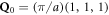 is the wavevector for simple G-type antiferromagnet and
  is the pseudo-cubic lattice constant. Hence, the ordering wavevectors are
  ,
,  , and
, and  . In terms of
  , the cycloidal period is
  .
.
FE and AF distortions create the DM interactions  and
and  . Including all magnetic anisotropies produced by these distortions, the spin Hamiltonian can be written


where  and
and  represent nearest and next-nearest neighbor spins, respectively. This is the most general Hamiltonian that includes the allowed distortions in R3c BiFeO3 but neglecting exchange anisotropy terms of the form

which are usually small for transition metal ions with half-filled d-shell such as Fe3+. Moreover, due to the long wavelength of the cycloid, exchange anisotropy can be effectively absorbed into the single-ion anisotropy (SIA)  , which favors spin alignment along
  . All terms in this Hamitlonian are also essential to explain the spin modes of BiFeO3 observed using THz spectroscopy [21, 22].
Since the FE distortion is uniform, the  sum is translation invariant. Due to the translation-odd
  [111] AF octahedral rotation, the
  sum contains the coefficient
  , which alternates from one hexagonal layer
  to the next. Simplified forms for the DM terms
  and
and  are given in appendix
By ignoring the higher cycloidal harmonics but including the tilt [23] τ produced by  , the classicsl spin state can be approximated [24] as


so that the spins on each hexagonal layer depend only on the integer  . The weak FM moment
  of the canted antiferromagnetic phase above Hc is related to the tilt by [21]
  . For [5, 25]
  ,
,  or
or  . By comparison, the local spin-density approximation (LSDA)+U (U = 5 eV) calculations described in the next section yield
  . Because higher harmonics are neglected, averages taken with the tilted cycloid in zero magnetic field introduce a very small error of order 10−5. Quantum fluctuations about the classical spin state are expected to be small for
  Fe3+ ions.
2. First-principles method
First-principles calculations were performed using density functional theory (DFT) from the VASP code within LSDA+U. The Hubbard U = 5 eV and the exchange  parameters were optimized for Fe3+ in BiFeO3 [26, 27]. We employed projector augmented wave potentials [28, 29]. To integrate over the Brillouin zone, we constructed a supercell made of 2 × 2 × 2 perovskite units (40 atoms, 8 f.u.) and a 3 × 3 × 3 Monkhorst–Pack k-points mesh. The DM interactions
  and
and  were evaluated with 4 × 2 × 2 units (80 atoms, 16 f.u.) and a 1 × 3 × 3 Monkhorst–Pack mesh. The wave functions were expanded with plane waves up to an energy cutoff of 500 eV. To calculate exchange interactions (Jn), we applied four different magnetic configurations (G-AFM, C-AFM, A-AFM and FM). We estimated
  and
and  by replacing all except four of the Fe3+ cations with Al3+ [26] in the 80 atom unit cell. As shown in table 1, the LSDA+U results are in excellent agreement with recent neutron-scattering measurements [22].
Table 1.
Calculated magnetic interaction parameters (meV) compared to spin model results fitted to neutron-scattering measurements [22].  splits into two components parallel (A = 0.042) and perpendicular (B = 0.075) to spin bond direction. The components A and B are explained in appendix
| meV | J1 |

|

|
K |
|---|---|---|---|---|
| LSDA+U | −6.1 | 0.089 | 0.042, 0.075 | 3.5 × 10⁻³ |
| Neutron | −5.3 | 0.103 | 0.064 | 4.1 × 10⁻³ |
After obtaining the exchange, DM, and SIA interactions, we calculate their derivatives with respect to an applied electric field parallel to a cartesian direction. A dielectric constant  is used to estimate the SD polarizations when the electric field is perpendicular to the rhombohedral axis [30]. To simulate atomic displacements driven by the applied field Eα, we evaluate the lowest-frequency polar eigenvector from the dynamical matrix by forcibly moving the atoms incrementally from the ground state R3c structure. The resulting energy difference between the two structures is divided by the induced electric polarization
  . The major difference in the polar eigenvectors obtained from the dynamic and the force-constant matrices arises from the Fe–O–Fe bond angle. The eigenvectors of the dynamic matrix reduce the bond-angle while the eigenvectors of the force-constant matrix raises that angle (see appendix
3. SC polarizations
The cross products  modulate the Fe–O–Fe bond angle and produce the SC polarizations [31]. These SC polarizations are simply obtained from electric-field derivatives of Dzyaloshinskii–Moriya interaction Hamiltonian. In BiFeO3, FE and AF distortions generate SC polarizations
  and
and  associated with the electric-field derivatives of the DM interactions
  and
and  . These are calculated using the procedure described in [20].
The first SC polarization is induced by the response of the FE distortion to an external electric field:

where  is a sum over nearest neighbors with
  and
and  ,
,  , or
, or  cubic axis. The electric-field derivatives of the DM interactions
  are given in appendix
  of
of  between spins
  and
and  with
with  parallel to the electric field is parallel to
  , the derivative
  (
( ) of
) of  between spins with
  perpendicular to the electric field is perpendicular to
  , as shown in figure 1.
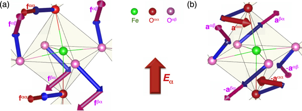
Figure 1. Influence of electric fields on the DM interactions. Blue arrows denote DM vectors without  and red arrows denote the change of the DM interactions with
  . (a) FE-induced DM (
 ) and its derivative vectors (
 ) with respect to
  . (b) AF-induced DM (
 ) and its derivative vectors (
 ) with respect to
  . The signs of the vectors alternate due to the AF rotations. Thick- and light-red arrows denote responses of DM to
  along the α direction when bonds between Fe ions are parallel (
 ,
,  ) and perpendicular (
 ,
,  ) to
) to  , respectively. The size of the arrows is proportional to the magnitude of the response to
  . O
. O (O
(O ) denotes oxygens along bonds parallel (perpendicular) to
  . Bi atoms are not drawn for clarity.
Download figure:
Standard image High-resolution imageTable 2.
SD polarizations from ES, SC and SIA. Shown are the calculated (LSDA+U) electric-field derivatives of J1,  , and K. The upper left and right scripts denote the directions of the spin bond and electric field, respectively.
  ,
,  , and
, and  by R3c symmetry as in appendix
  . All units are nC cm−2.
SC polarization from 
|
SC polarization from 
|
ES polarization from J1 | |||||
|---|---|---|---|---|---|---|---|

|

|

|
 + 2 + 2 |

|

|

|
|
| LSDA+U | 9 | 17 | 14 | 17 | −19 | −250 | −350 |
| NDD | 36 | 29 | 29 | 28 | −7.2 | — | — |
In the lab reference frame  , regrouping terms for domain 2 with
 ![${{\bf{x}}}^{\prime }=[1,0,-1]$](https://content.cld.iop.org/journals/1367-2630/18/4/043025/revision1/njpaa1bccieqn115.gif) using equations(7)–(9) yields
using equations(7)–(9) yields

where

with  ,
,  , and
, and  given in table 2. Fits to the NDD [19] described in section 6 imply that g = h.
The second SC polarization alternates in sign due to the alternating AF rotations along [111]:

The SC polarization components  are evaluated in table 2. While the derivative
  of
of  between spins
  and
and  with
with  parallel to the electric field is nearly anti-parallel to
  , the derivative
  (
( ) of
) of  between spins with
  perpendicular to the electric field is perpendicular to
  , as shown in figure 1.
Appendix

where

with  and
and  given in table 2.
4. ES polarizations
The absence of an inversion center between neighboring spin sites induces the ES bond polarizations. Since the scalar product  is altered by external perturbations such as temperature, electric field, or magnetic field, FE and AF distortions each generates its own ES polarization.
For symmetric exchange couplings, ES is dominated by the response of the nearest-neighbor interaction J1:

The two ES polarizations  and
and  are closely related to one another. The electric-field derivatives
  are given in the cubic coordinate system by


where  (
( ) and
) and  for spin bonds perpendicular and parallel to the electric field, respectively.
Because the AF octahedral rotation is perpendicular to  , the ES polarization associated with AF rotations is also perpendicular to
  with
with


Unlike W1u, W2u alternates in sign due to the opposite AF rotations on adjacent hexagonal layers.
The first ES polarization parallel to  with coefficient
  modulates the FE polarization that already breaks IS above
  . The second ES polarization perpendicular to
  has coefficient
  . The AF rotations affect the bonds between nearest-neighbor spins in the plane normal to
  because each oxygen moves along the directions
 ![$[0,-1,1]$](https://content.cld.iop.org/journals/1367-2630/18/4/043025/revision1/njpaa1bccieqn150.gif) ,
, ![$[1,0,-1]$](https://content.cld.iop.org/journals/1367-2630/18/4/043025/revision1/njpaa1bccieqn151.gif) , and
, and ![$[-1,1,0]$](https://content.cld.iop.org/journals/1367-2630/18/4/043025/revision1/njpaa1bccieqn152.gif) , perpendicular to
, perpendicular to  . Thus, the second ES polarization is associated with atomic displacements perpendicular to
  and parallel to the AF rotation.
Figure 2 demonstrates the strong anisotropy in the response of magnetic exchange to an electric field. While  arises from the change in Fe–O–Fe bond angle due to a polar distortion,
  arises from bond contraction. As shown,
  is much more sensitive to an electric field than
  . Since the ME anisotropy
  produces an ES polarization, the AF rotation angle is changed by the spin ordering. In particular, the negative sign of
  nC cm−2 indicates that the rotation angle increases with the dot product
  because oxygen atoms moving in the AF plane have a negative effective charge
  .
.
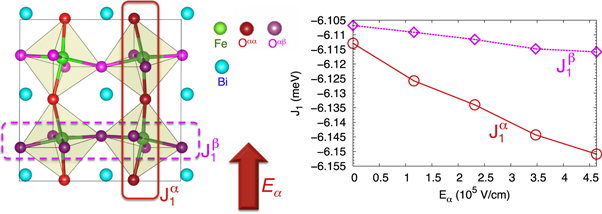
Figure 2. Strong anisotropic response of magnetic exchange (J1) to an electric field. The slopes of thick and dotted lines represent derivatives of J1 with respect to electric fields parallel ( ) and perpendicular (
 ,
,  ) to the spin-bond direction calculated from DFT.
Download figure:
Standard image High-resolution imageThe anisotropic ES polarization components  and
and  cooperatively induce the ES polarization along
  under the IS broken by the FE polarization. In contrast to our previous study [20] on the response to a static electric field (
 nC cm−2), we obtain a negative
  nC cm−2 in a dynamic electric field. Appendix
  increases the bond angle of Fe–O–Fe (positive
  ) but a dynamic
  decreases the bond angle (negative
  ) due to the Goodenough–Kanamori rules [32].
We recently predicted [20] that the static SD polarization of BiFeO3 is about −3 μC cm−2 along a cubic diagonal opposite to the FE polarization emerging below  . The electronic plus atomic contribution to the SD polarization is −1.3 μC cm−2 and the lattice-deformation contribution is −1.7 μC cm−2, which were slightly underestimated (−1.0 and −1.3, respectively) in previous literature [33, 34]. The total SD polarization (−3 μC cm−2) is higher than observed in any other known multiferroic material [20].
5. Origin of NDD
The most stringent test yet for the microscopic model proposed above is its ability to predict the NDD which is the asymmetry  in the absorption
  of light when the direction of light propagation is reversed. The absorption of THz light is given by
  , where [35, 36]

is the complex refractive index for a linearly polarized beam,  ,
,  and
and  are the dielectric, magnetic, and magnetoelectric susceptibility tensors describing the dynamical response of the spin system [13, 15, 17, 35] and
  is the dielectric constant related to the charge response. Subscripts i and j are fixed by the electric
  and magnetic
  polarization directions, respectively. The second term, which depends on the light propagation direction and produces NDD, is separated from the mean absorption by writing
  .
.
Summing over the spin-wave modes n at the cycloidal ordering wavevector  ,
,  is given by


where  is the magnetization,
  is the volume per Fe site,
  is the net SD polarization given in units of, nC cm−2, and
  .
.
For each field orientation, the integrated weight of every spectroscopic peak at  is compared with the measured values, thereby eliminating estimates of the individual peak widths. Experimental results for the NDD with field along
 ![${\bf{m}}=[1,-1,0]$](https://content.cld.iop.org/journals/1367-2630/18/4/043025/revision1/njpaa1bccieqn193.gif) are plotted in figure 3(a) for
are plotted in figure 3(a) for ![${\bf{e}}=[1,-1,0]$](https://content.cld.iop.org/journals/1367-2630/18/4/043025/revision1/njpaa1bccieqn194.gif) . Fits to the NDD are based on the plotted 2, 4, 6, 8, 10, and 12 T data sets. For each data set, we evaluate the integrated weights for the eight modes [22]
. Fits to the NDD are based on the plotted 2, 4, 6, 8, 10, and 12 T data sets. For each data set, we evaluate the integrated weights for the eight modes [22]  ,
,  ,
,  ,
,  , and
, and  between roughly 12 and 35 cm−1.
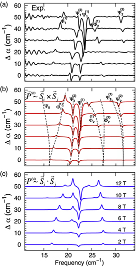
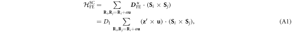
Figure 3. Origin of the strong NDD in BiFeO3. (a) The experimental NDD (Δ α) with static magnetic field from 2 to 12 T and oscillating electric field along ![$[1,-1,0]$](https://content.cld.iop.org/journals/1367-2630/18/4/043025/revision1/njpaa1bccieqn200.gif) . The predicted NDD using (b) SC and (c) ES polarizations. Here,
. The predicted NDD using (b) SC and (c) ES polarizations. Here,  denote nearest neighbors.
Download figure:
Standard image High-resolution imageComparing figures 3(a) and (b), the NDD for ![${\bf{m}}=[1,-1,0]$](https://content.cld.iop.org/journals/1367-2630/18/4/043025/revision1/njpaa1bccieqn202.gif) is dominated by the two sets of SC polarizations
is dominated by the two sets of SC polarizations  and
and  . Table 2 indicates that the fitting results are not significantly changed by including the ES polarizations. Figure 3(c) attempts to fit the experimental data using the ES polarizations alone. Clearly, the ES polarizations by themselves cannot produce the observed NDD.
Figures 3(a) and (b) indicate that the various components of the SC polarizations in BiFeO3 are captured by first-principles calculations and that the NDD is not strongly affected by the ES terms This selectivity originates from the spin dynamics of this nearly collinear antiferromagnet. Due to the very small SIA on the S = 5/2 Fe3+ spins, each magnon mode can be described as the pure precession of Fe3+ spins: the oscillating component  of the spin on site i is perpendicular to its equilibrium direction
  . Since neighboring spins in the long-wavelength spin cycloid of BiFeO3 are close to collinear, a dynamic polarization is effectively induced by SC terms such as
  . However, the dynamic polarization generated by ES terms
  is almost zero. The spin stretching modes observed in strongly anisotropic magnets [35, 38] do not appear in BiFeO3.

Figure 4. Distinct atomic responses to dynamic and static electric fields. The lowest-frequency eigenvectors of (a) dynamic and (b) force-constant matrices are compared. Note that the polar displacement in the dynamic limit (ω = 78 cm−1) increases the Fe–O–Fe bond angle (dotted line) while the displacement decreases the bond angle in the static limit.
Download figure:
Standard image High-resolution image
Recent work [37] explains the observed static polarization perpendicular to  by the
  term proportional to h − f. Although the fitting and LSDA+U values for
 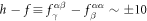 nC cm−2 in table 2 are an order of magnitude smaller than required by that work, keep in mind that the SC parameters given in table 2 were evaluated or fitted for a dynamic electric field.
Although DFT calculations underestimate the ME coefficients compared to the NDD fitting results in table 2, they nicely demonstrate which of the symmetry-allowed ME couplings are relevant and which are negligibly small. Combining the two methodologies allows a more unambiguous determination of these coupling parameters. There are several possible explanations for the difference between the results obtained from DFT calculations and the NDD fitting. First, a larger dielectric constant  could produce better agreement between DFT and NDD since the SD polarizations are proportional to
  through

Second, higher-frequency polar modes not considered here also can affect NDD. Third, a smaller Hubbard U will increase the SD polarizations and improve the agreement with the experimental fits. Fourth, magnon modes were observed between  and 40 cm−1 while we calculated the SC coupling constants in the dynamical limit. The crossover frequency
  between static and dynamical behavior lies between 0 and the polar phonon at
  cm−1. If
  lies in the middle of the measured frequencies, then the SC fitting parameters may differ from the dynamical couplings obtained from LSDA +U.
6. Discussion
In order to study the ME couplings in complex multiferroic systems, first-principles calculations must be anchored to the right microscopic Hamiltonian. With two sets of SC polarizations derived from the two distinct structural distortions, BiFeO3 is a good example of how our atomistic approach works for complex materials. This paper calculated only the ionic displacement contribution to the ME coupling which is typically larger than the purely electronic contribution [34, 39]. The lattice deformation contribution to the SD polarization was discussed in our previous work [20].
The higher-frequency polar modes contribute to the electric-field induced displacement. Their contributions are proportional to the mode strength  , where Z is the mode effective charge and ω its frequency. From our dynamical matrix calculations, the mode strengths of the higher frequency modes are less than 30% smaller than the strength of the lowest mode. Therefore, the lowest mode makes dominates the electric-field induced polar displacement.
The advantages (large FE polarization, high  , and high
  ) of BiFeO3 are also major obstacles to understanding the ME couplings that produce the SD polarizations below
  . Leakage currents and the preexisting large FE polarization at high temperatures have hampered magneto-capacitance measurements and hidden the SD polarizations. Although recent neutron-scattering measurements [10] imply a large ES polarization, most other ME polarizations are unknown. We show that NDD measurements combined with first-principles calculations based on a microscopic model reveal the hidden SC polarizations. In particular, this approach allows us to disentangle the delicate SC polarizations and the hidden ES polarizations associated with AF rotations. We envision that intrinsic methods such as NDD will reveal hidden ME couplings in many materials and rekindle the investigation of type-I multiferroics.
Acknowledgments
We acknowledge discussions with H Kim, E Bousquet, Nobuo Furukawa, S Miyahara, J Musfeldt, U Nagel, S Okamoto, S Bordács and T Rõõm. Research sponsored by the US Department of Energy, Office of Basic Energy Sciences, Materials Sciences and Engineering Division. IK was supported by the Hungarian Research Fund OTKA K 108918. JHL was in part supported by the year of 2015 Research Fund (1.150132.01) of the UNIST (Ulsan National Institute of Science and Technology). We also thank Hee Taek Yi and Sang-Wook Cheong for preparation of the BiFeO3 sample.
Appendix A.: Simplified form for the Dzyaloshinskii–Moriya interactions
A.1. FE-induced Dzyaloshinskii–Moriya interaction
Since the FE vectors  are given by (0,
  ,
,  ), (
), ( ,
,  , 0), and (
 ,
,  , 0) between nearest spins along
  ,
,  , and
, and  , respectively, the FE-induced DM interaction can be transformed as:
where  meV is now larger by
  than in previous work [21].
A.2. AF-induced Dzyaloshinskii–Moriya interaction
The AF interactions  along
along  ,
,  , and
, and  can be written


For domain 2 with ![${{\bf{x}}}^{\prime }=[1,0,-1]$](https://content.cld.iop.org/journals/1367-2630/18/4/043025/revision1/njpaa1bccieqn238.gif) ,
,
where the primed sum over  is restricted to either ni odd or even hexagonal layers. Based on the tilted cycloid of equations (7)–(9) the
  term dominates because
 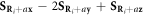 is of order
  .
.
Previously, the second DM term was written
which also uses equations (7)–(9). Therefore,  meV, which is in excellent agreement with previous work [21].
Appendix B.: Eigenvectors of dynamic and force-constant matrices
As noted in section 4,  is negative from the eigenmode of the dynamic matrix while it is positive from the eigenmode of the force-constant matrix [20]. This difference originates from the opposite changes to the Fe–O–Fe bond angle: the bond angle increases in the static limit while it decreases in the dynamic limit.
Appendix C.: Spin-current polarization components
Defining  ,
,


where  , and
, and  .
.
Defining  ,
,


where  , and
, and  .
.
Appendix D.: SC polarization from antiferrodistortive Dzyaloshinskii–Moriya coupling
For domain 2 with ![${{\bf{x}}}^{\prime }=[1,0,-1]$](https://content.cld.iop.org/journals/1367-2630/18/4/043025/revision1/njpaa1bccieqn251.gif)

which use

The SD polarization associated with  is
is


Similarly


So in the local frame


plus a correction of order  .
.
The polarization matrix used to evaluate the NDD is given by

where  nC cm−2 and
  nC cm−2 are obtained from first principles as given in table 2. (
 nC cm−2,
  nC cm−2,
  nC cm−2,
  nC cm−2, and
  nC cm−2).
Footnotes
- *
This manuscript has been written by UT-Battelle, LLC under Contract No. DE-AC05-00OR22725 with the US Department of Energy. The United States Government retains and the publisher, by accepting the article for publication, acknowledges that the United States Government retains a non-exclusive, paid-up, irrevocable, world-wide license to publish or reproduce the published form of this manuscript, or allow others to do so, for United States Government purposes. The Department of Energy will provide public access to these results of federally sponsored research in accordance with the DOE Public Access Plan.