


Abstract
Protein molecular motors play a fundamental role in biological cells and development of their synthetic counterparts is a major challenge. Here, we show how a model motor system with the operation mechanism resembling that of muscle myosin can be designed at the concept level, without addressing the implementation aspects. The model is constructed as an elastic network, similar to the coarse-grained descriptions used for real proteins. We show by numerical simulations that the designed synthetic motor can operate as a deterministic or Brownian ratchet and that there is a continuous transition between such two regimes. The motor operation under external load, approaching the stall condition, is also analysed.
Export citation and abstract BibTeX RIS

Original content from this work may be used under the terms of the Creative Commons Attribution 3.0 licence. Any further distribution of this work must maintain attribution to the author(s) and the title of the work, journal citation and DOI.
Introduction
Single-molecule motors play a fundamental role in biological cells. If their synthetic analogues are developed and implemented, this may lead to exciting technological applications. Because of their importance, protein motors are currently subject of intensive experimental and theoretical investigations. High-precision single-molecule experiments with myosin [1, 2], kinesin [3, 4], F1-ATPase [5, 6], hepatitis C virus (HCV) helicase [7–9] and other motor proteins have been performed; they have yielded valuable information about the details of their operation. Since chemical structures of these molecules are known, their behaviour can also be studied by direct all-atom molecular dynamics (MD) simulations. The difficulty involved in MD simulations is that they are extremely time-consuming and, for typical protein motors, only the dynamics on the scales of up to a microsecond could have been resolved in such simulations. Taking into account that a single turnover cycle of a molecular motor would usually take about 10 ms, it is obvious that full MD simulations are still far from reproducing even single motor operation cycles (though they can indeed strongly contribute to clarification of the details of such cycles).
There are two ways to overcome this difficulty. On the one hand, special hardware for accelerated MD simulations is being developed. By using the specialized ANTON hardware, it has already become possible to follow the dynamics of a small protein, the bovine pancreatic trypsin inhibitor (BPTI), over the time span of 1 ms [10]. Soon, such simulations may already become feasible for the larger proteins. However, running an all-atom simulation over many turnover cycles for an actual molecular motor, with all reaction events included, and accumulating the data for statistical analysis over many such cycles would remain a distant challenge for MD simulations even in the future.
On the other hand, coarse-grained protein models can be employed to speed up the simulations. While many variants, such as, e.g., the Go-model [11, 12] , are available, the attention has recently become focused on the class of elastic-network (EN) models. In the anisotropic EN model, introduced by I. Bahar with coworkers in 2001 [13], a protein is treated as a network of point particles (residues) with elastic interactions between network neighbours. The network is built by using the experimental x-ray diffraction information about the equilibrium structure of a protein.
While EN models are empirical and could not so far be derived from the full dynamical models, it has been checked that, for many proteins, they correctly reproduce thermal fluctuations in the positions of residues (B-factors) in the framework of the normal-mode analysis [14–19]. Moreover, they can be used to explore sensitivity of the proteins to local perturbations, such as binding of a ligand [20–22]. The EN models have been already applied to principal molecular motors, such as myosin V or kinesin [23–27]. Details of EN applications can be found in the review volume [28] with the foreword by Karplus. In a recent publication [10], predictions of an EN model were compared with the data from a 1 ms ANTON simulation for the BPTI protein and good agreement has been observed. Improvements of the original elastic EN model have been proposed and investigated (see, e.g., [29–32]).
Using reduced EN descriptions, it already becomes possible to trace entire operation cycles of real protein machines and molecular motors. For the enzyme adenylate kinase, complete turnover cycles including the solvent effects could be reproduced and statistical analysis for the sequences of many such cycles could be performed [33]. For the molecular motor HCV helicase, single turnover cycles could be traced and interactions of this motor with the double-stranded DNA could be resolved [34], confirming the inchworm ratchet mechanism deduced from the experiments [35].
In addition to structurally resolved theoretical studies of protein motors, based on either full MD or reduced EN simulations, there are also investigations where the internal dynamics of a molecular motor is not resolved. Instead, the entire motor is modelled as a particle moving in a periodic potential. The theoretical concept of a molecular motor as a Brownian ratchet has attracted much attention [36–41]
Different kinds of synthetic nanomotors have been previously proposed and investigated. Sometimes, micrometer-size particles are referred to as the 'motors' if they can propel themselves through a fluid due to the imbalance of surface tension forces (see, e.g., [42]). It has been conjectured that even single enzyme molecules, when catalytically active, can generate propulsion forces and actively move in the solution [43, 44]. A different kind of motors are swimmers that can actively move in fluids [45] and lipid bilayers [46] by actively changing their conformation or based on other molecular interactions [47]. Furthermore, relatively small molecules operated as switches are able to move actively and thus to behave as motors too (see review [48] ). Such kinds of motors, however, differ in their operation mechanisms from protein machines.
The aim of the present study is twofold. First, we demonstrate how a model molecular motor, roughly resembling the properties of real protein machines and, in particular, of the muscle myosin, can be constructed. Second, we perform extensive statistical analysis of this model EN motor. The mean propagation velocity as a function of the temperature parameter, controlling the intensity of fluctuations is determined. The motor operation under load is moreover considered. By varying the parameters, we show that the same model can be operated in the weak and strong coupling regimes which correspond to deterministic and Brownian ratchets; the intermediate regimes are also possible. Investigations of such model system can help to better understand the operation of real protein motors and, furthermore, they can assist in the future physical implementation of synthetic molecular motors similar in their functional principles to their actual biological counterparts.
Results
The elastic machine
The proposed model motor consists of a cyclically operating machine that interacts with the filament by employing a ratchet mechanism which transforms cyclic machine movements into the translational motion of the filament. First, we explain how the machine is designed. Its interactions with the filament are described in the next section.
The EN machine which we use has been proposed by Togashi and Mikhailov [23] and has previously been employed in other applications [49–51]. Nonentheless, only a brief description of the machine has so far been provided [23]. It has been designed [23] by using evolutionary optimization methods, in such a way that its conformational dynamics and ligand-induced internal motions closely resemble those of actual protein machines. Particularly, its equilibrium states, with and without the ligand, have large attraction basins, so that even after large perturbations the system returns back to them. Moreover, relaxation proceeds along a well-defined path in the conformational space.
The model machine is made up of two relatively rigid domains connected by a flexible hinge region (figure 1). A substrate ligand can bind in a binding pocket situated in the hinge region and induce a closing motion of the domains about the hinge. Furthermore, the substrate ligand can get converted to the product and get released, thus bringing about the reverse opening hinge motion. The machine has 64 identical particles connected by a set of identical elastic links.

Figure 1. Elastic network of the machine. The network is formed by 64 particles (green and blue beads) connected by elastic links. Additionally, the ligand (red bead) and its links to the three binding nodes  (blue beads) are shown.
Download figure:
Standard image High-resolution imageThe elastic energy of the machine is given by

Here  is the set of all coordinates
  of the particles
  . κ is the elastic constant which is the same for all the elastic links in the network. The network architecture is specified by the adjacency matrix whose elements Aij are either 1 or 0 depending on whether a bond exists between a pair of particles i and j. Furthermore,
  is the distance between the pair of particles i and j, and
  is the equilibrium distance between them;
  are equilibrium positions of all the nodes. The equilibrium positions
  of the particles and the matrix of connections Aij are given in [23] (see also methods).
The machine operates inside a viscous fluid. Its dynamics is overdamped and is described by the equations

where γ is the mobility coefficient, the same for all beads  . Later, thermal fluctuations will be taken into account by introducing noise terms into such relaxation equations. Note that inertial effects can also be neglected for real protein machines, when conformational motions on the time scales larger than a picosecond are considered. Hydrodynamic effects are not treated in the present study, but they can be included too [49].
When the ligand binds, it forms elastic links with three beads ( located in the hinge area. The ligand itself is treated in our model as an additional particle (i = 65). It is convenient to introduce a binary variable s which takes the value s = 1, if the ligand is attached, and s = 0 otherwise. The expression for the elastic energy, including the ligand at the position
  , is
, is

The last ligand interaction term depends on the distances  between the ligand and the three network beads. Moreover,
  are the natural lengths of the three additional links,
 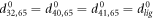 . For simplicity, we assume that the ligand links have the same elastic constant κ as the other links in the network. When the ligand is present, the network dynamics is given by equations (2) where the expression (3) for the elastic energy should be used.
Next, the conditions at which binding or release of the ligand take place need to be specified. Moreover, the initial position of the ligand after binding should also be defined. In the present study, we use the ligand binding and detachment conditions which are slightly different from the original formulation [23] and are defined in terms of the hinge angle; such conditions have already been employed in the study of membrane machines [51]. The hinge angle ϕ is introduced through the equation

Where  is the centre of mass of the three beads
  and 41 which form the ligand binding pocket

Because the two arms of the machine are fairly stiff, the angle ϕ can be interpreted as the angle between the two arms (see figure 2).
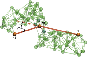
Figure 2. Definition of the hinge angle ϕ. Here, cm denotes the centre of mass of the three ligand binding particles  .
.
Download figure:
Standard image High-resolution imageIn the equilibrium state of the ligand-free network the hinge angle is relatively large ( ) and we refer to this state as the open conformation of the machine. We assume that binding of the substrate ligand is possible within a certain interval
 ![$[{\phi }_{0}-{{\rm{\Delta }}}_{0},{\phi }_{0}+{{\rm{\Delta }}}_{0}]$](https://content.cld.iop.org/journals/1367-2630/18/4/043006/revision1/njpaa1c2eieqn19.gif) of hinge angles in the vicinity of the open conformation. Within this interval, it can take place with some transition probability w0 per unit time. We assume that, when the ligand arrives, it becomes located in the centre of mass of the binding pocket formed by the particles
of hinge angles in the vicinity of the open conformation. Within this interval, it can take place with some transition probability w0 per unit time. We assume that, when the ligand arrives, it becomes located in the centre of mass of the binding pocket formed by the particles  hence we have
  at the moment of binding.
The ligand-network complex will undergo relaxation to its own equilibrium state. This relaxation process will be described by equations (2) where the expression (3) for the elastic energy with s = 1 should be used. Note that, when the ligand is attached to the network, it moves like any other particle; we assume for simplicity that its mobility γ is the same.
When designing the machine, the natural lengths of the ligand links are chosen to be shorter than their typical initial lengths. Therefore, these links tend to shrink. Note that, through the ligand located in the hinge region, the two arms become additionally linked. When the ligand links get shorter, the two arms move closer one to another and the hinge angle decreases. The equilibrium state of the ligand-network complex corresponds therefore to a closed conformation of the machine which is characterized by a relatively small hinge angle  .
.
Figure 3 displays the operation cycle of the designed elastic machine. At the beginning of the cycle (figure 3(a)) the machine is in an open conformation. The substrate ligand (red particle) arrives into the ligand binding pocket in the hinge region and establishes elastic links (figure 3(b)) to three neighbouring beads (blue colour). This induces a transition to the the closed conformation (figure 3(c)) which corresponds to the equilibrium state of the ligand-machine complex. Now the ligand is converted to the product particle which is instantaneously released (figure 3(d)). After that the free machine returns to its equilibrium open conformation and the cycle can be repeated. The detailed operation of the machine can be observed in video 1.

Figure 3. Operation cycle of the machine.
Download figure:
Standard image High-resolution imageThe reaction is introduced by assuming that in the vicinity of the closed conformation the nature of the bound ligand can suddenly change, so that it gets transformed to a product particle which is immediately released. This transition occurs with the probability w1 per unit time within the interval ![$[{\phi }_{1}-{{\rm{\Delta }}}_{1},{\phi }_{1}+{{\rm{\Delta }}}_{1}]$](https://content.cld.iop.org/journals/1367-2630/18/4/043006/revision1/njpaa1c2eieqn23.gif) of the hinge angle. The release of the product is characterized by sudden disappearance of the three elastic links between the ligand and the network. After the transition the elastic energy of the network is described by equation (3) with s = 0. As we assume, the product is immediately evacuated and therefore the reverse binding of the product to the machine cannot occur. We also neglect the possibility that the substrate dissociates before it gets converted to the product.
of the hinge angle. The release of the product is characterized by sudden disappearance of the three elastic links between the ligand and the network. After the transition the elastic energy of the network is described by equation (3) with s = 0. As we assume, the product is immediately evacuated and therefore the reverse binding of the product to the machine cannot occur. We also neglect the possibility that the substrate dissociates before it gets converted to the product.
Interactions with the filament
Our aim is to imitate some aspects of the functioning of a real molecular motor, the muscle myosin. In each of its cycles, the myosin performs a power stroke, induced by binding of ATP and the hydrolysis reaction. Under the power stroke, the myosin head is attached to the actin filament and generates a force to drag it. After the power stroke the head gets detached and the protein returns to its initial conformation. Because the myosin holds the filament during the forward part of the cycle and is detached from it during the backward part, a ratchet effect is naturally implemented. As we will show, similar operation can be achieved by using the elastic machine described in the previous section. Note, however, that an important aspect of myosin motor operation would still be absent in our model. The myosin actively grasps the actin filament, because of the conformational changes in the actin binding cleft that are ligand-induced. Our model is too primitive to incorporate such a mechanism. Instead, a different interaction between the motor and the filament will be employed.
Before we proceed to the detailed formulation, we want to show how the motor would work. Video 2 gives an example of the motor operation in absence of thermal fluctuations. When the ligand binds, a power stroke is executed. As the machine moves forward approaching its closed conformation, the swinging arm comes very near the filament and establishes an attractive bond with it, thereby dragging the filament forward. While holding the filament, it moves forward, until the ligand conversion into the product and its release occur. In the second part of the cycle, when the machine returns to its equilibrium open conformation, the swinging arm moves along a path farther away from the filament and no attractive bond is formed, so the machine and the filament stay detached from each other.
Figure 4(a) illustrates the set-up of our model. As shown in figure 4(a), the filament is positioned along the x-axis of our chosen coordinate system. It can only move back or forth along this axis. The swinging free arm of the elastic machine is assumed to have a special node (i = 64) that can interact with the filament. The other arm of the machine is immobilized by fixing the nodes,  at
at  ,
,  and
and 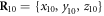 .
.
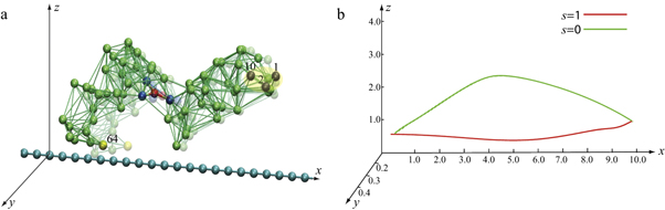
Figure 4. (a) Construction of the motor system. Three beads  are immobilized. The bead i = 64 interacts with the regularly spaced force centres of the filament which is free to move along the x-axis. (b) The trajectory of the node i = 64 for one operation cycle.
Download figure:
Standard image High-resolution imageThe trajectory of the end particle (i = 64) of the machine as it undergoes cyclic conformational changes is displayed in figure 4(b). The trajectory of the end particle is an almost planar loop, lying approximately on the x-z plane. Figure 5(a) shows the time dependence of the distance h64 of the interacting node from the filament. For the chosen position of the machine, the end particle remains close to the filament during the forward part of the cycle (s = 1) while it is relatively far away during the reverse part (s = 0). Additionally, figure 5(b) shows the time dependence of the position x64 of the end particle along the filament. During the power stroke (s = 1), the arm moves in the forward direction, whereas the reverse motion occurs during the rest of the operation cycle for the motor.
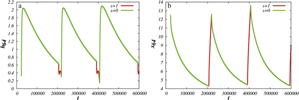
Figure 5. (a) Time dependence of the distance h64 between the interacting node and the filament. (b) Time dependence of the position x64 of the interacting node on the x-axis along the filament. Distances are measured in units of  .
.
Download figure:
Standard image High-resolution imageNote that the time of the power stroke is much shorter than the time needed for the arm to return to its initial position. This is because, during the power stroke, additional attractive interactions between the arm and the head of the machine are present through the ligand located in the hinge.
Real actin filaments are formed by a periodic linear arrangement of monomers representing single actin proteins. In our model system, we do not want to reproduce such complex structure. Instead, it is assumed that the filament represents a rigid rod whose motions are constrained to a line chosen as the x-axis in our coordinate frame. Along the filament, periodically spaced force centres are located. Their positions are

where a is the spatial period and X(t) is the coordinate of the entire rigid filament at time t. Each of the force centres is capable of interacting with the machine tip.
To model the interaction between the filament and the machine tip, Lennard–Jones potentials are used. The total interaction potential  between the end particle (
 of the machine and the filament is given by a sum of pair interation potentials

where

and

Here  is the distance between the end particle (i = 64) and the nth force centre of the filament,
 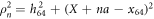 . The coefficient σ specifies the interaction strength, while the parameters C and lc determine the range of the interaction.
Note that the interaction potential is a periodic function of the filament position X and it has the period a. Indeed, the total interaction with the (infinite) filament is not changed if the filament is shifted by distance a corresponding to the separation between individual force centres. Figure 6 shows the interaction potential (equation (7)) as a function of the filament position X for three different distances h64. The periodicity of the effective interaction potential is determined by the lattice distance a, of the force centres on the filament.
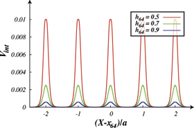
Figure 6. Profiles of the interaction potential Vint in units of  for different separations h64 of the interacting node (i = 64) from the filament. Separations are measured in units of
  .
.
Download figure:
Standard image High-resolution imageThe complete model
Thus, the equations of motion for the particles ( ) of the motor and the filament have the form


Here  is the elastic energy (3) of the machine and
  in the interaction given by equation (7). The mobilities of the machine particles and of the filament are γ and Γ, respectively. We have added to the last equation the external force Fext which may be applied to the filament.
The last terms in the equations (10), (11) and (13) take into account thermal fluctuations. In equations (10) and (11) ,  are independent white vector noises having the correlations

kB is the Boltzmann constant and T is the temperature. In equation (13)  is a white noise with the correlation function

The discrete variable s takes two values : s = 0 corresponds to the free machine, whereas s = 1 corresponds to the ligand-bound machine. Binding of the ligand, i.e., transition from s = 0 to s = 1, is a stochastic event which takes place with the probability rate w0 within the interval ![$[{\phi }_{0}-{{\rm{\Delta }}}_{0},{\phi }_{0}+{{\rm{\Delta }}}_{0}]$](https://content.cld.iop.org/journals/1367-2630/18/4/043006/revision1/njpaa1c2eieqn41.gif) of the hinge angle given by equation (4). The release of the ligand, i.e., transition from s = 1 to s = 0, can take place with the probability rate w1 inside the interval
of the hinge angle given by equation (4). The release of the ligand, i.e., transition from s = 1 to s = 0, can take place with the probability rate w1 inside the interval ![$[{\phi }_{1}-{{\rm{\Delta }}}_{1},{\phi }_{1}+{{\rm{\Delta }}}_{1}]$](https://content.cld.iop.org/journals/1367-2630/18/4/043006/revision1/njpaa1c2eieqn42.gif) of the hinge angle. Note that generally the rates w0 and w1 depend on temperature T. In our model system, such possible dependence is not however taken into account. Our investigations will be always performed near to the saturation regime, with binding or release of a ligand always taking place once the respective window has been entered. The focus will be on the fluctuation effects controlled by the temperature parameter in the model.
of the hinge angle. Note that generally the rates w0 and w1 depend on temperature T. In our model system, such possible dependence is not however taken into account. Our investigations will be always performed near to the saturation regime, with binding or release of a ligand always taking place once the respective window has been entered. The focus will be on the fluctuation effects controlled by the temperature parameter in the model.
When s = 1, the machine includes a ligand particle (i = 65) and the equation of motion for this particle has the form

where  is given by equation (3). The ligand particle has the same mobility γ and is subject to the same kind of noise (equation (14)) as the machine particles. When the ligand arrives, i.e., at the moment of the transition from s = 0 to s = 1, its initial position is
  where
where  is given by equation (5). When the reverse transition from s = 1 to s = 0 takes place, the ligand is immediately removed and we do not track its position any further. A new ligand particle is bound to the machine as the substrate and removed from it as the product in each next operation cycle.
In our numerical simulations, the dimensionless form of the model is employed. To obtain it, time is measured in units of  whereas the coordinates
  and X as well as the distances h64 and x64 are measured in the units of
  where a is the spacing between consecutive force centres on the filament. Below the same notations are used for the rescaled variables. In the dimensionless form, the explicit evolution equations of the model are


where  and
and  ; we use the step function H(z) = 1 for z > 0 and H(z) = 0 for z ≤ 0. The dimensionless interaction strength coefficient is
  and the dimensionless characteristic interaction distance is
  . The coefficient
  is the ratio of the mobilities of the machine particles and the filament. The rescaled external force is
The rescaled equations include new noises  and
and  with the correlation functions


where Θ is the rescaled temperature given by  . Note that the transition rate constants for the binding and release of the ligand also become rescaled and the dimensionless transition rate constants are
  and
and  .
.
Examples of motor operation
When conversion of the substrate into the product is excluded, the ligand binds to the machine and stays indefinitely long within it. Therefore, the motor can only exhibit thermal fluctuations characteristic for its ligand-bound equilibrium state (s = 1). In video 3, we show a simulation of the motor in this case under relatively weak thermal noise ( ). The swinging arm of the motor gets attached to the filament and performs equilibrium thermal fluctuations together with it. As could be indeed expected under equilibrium conditions, no uni-directional movement of the filament is observed.
If the motor is still at equilibrium (no substrate conversion), but the temperature is increased ( ), the behaviour becomes different (see video 4). Now, the arm of the motor cannot firmly hold onto the filament and, as a result, the filament easily slides against it. In contrast to video 3, motions of the arm and the filament seem to be independent in this case.
The behaviour of the motor gets changed dramatically when the reaction, i.e., the conversion of the substrate into product, is included. Video 5 shows the motor operating under these conditions at a low level of thermal fluctuations ( ).
).
If the temperature is increased to  , it can be observed (Video 6) that the arm of the motor begins to slide against the filament, similar to what is seen in video 4. This means that in this case the motor can only weakly affect the intrinsic independent Brownian motion of the filament.
Figures 7(a) and (b) display trajectories of the bead i = 64, located at the end of the arm, in the plane of the variables h64 (distance to the filament) and ϕ (hinge angle) at two temperatures  and
and  , respectively. Here, the red colour indicates that the ligand is present inside the machine (s = 1) and the green colour corresponds to the free machine (s = 0). For comparison, we also show in figure 7(c) the trajectories in absence of thermal noise, i.e.,
  . For each temperature, the data for 10 consecutive cycles is taken. Examining figures 7(a) and (b), one can notice that the motor arm is persistently cycling in a counter-clockwise direction. We can also notice that even at the relatively high temperature (
 ) in figure 7(b) the motions of the arm remain well-defined, so that the two branches with s = 0 and s = 1 do not overlap.
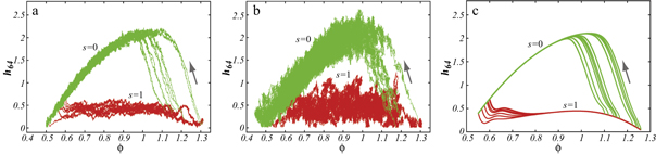
Figure 7. Trajectories of the bead i = 64 in the plane of variables h64 and ϕ at temperatures (a)  (b)
(b)  and (c)
  . The data for 10 consecutive cycles is taken.
Download figure:
Standard image High-resolution imageStrong and weak coupling regimes
Suppose first that the motor arm is fixed, so that the distance of the bead i = 64 from the filament, h64, and the projection of its position on the filament, x64, are both constant. Then the filament is effectively performing thermal Brownian motion in a periodic potential  . This potential is given by equation (22) and displayed for three different values of h64 in figure 6. As seen in figure 6, the height of the barrier strongly depends on the distance (h64) between the arm and the filament. At the typical distance,
  , which is characteristic for the ligand-bound state (s = 1), the barrier height is about
  . When the ligand is absent (s = 0), the separation gets increased above
  and, at such distances the interaction potential Vint vanishes. This means that in the ligand-free state the motor cannot exhibit any action on the filament.
Suppose now the motor arm moves in such a way that its separation from the filament h64 remains constant, but its position x64 with respect to the filament changes,  . Then the filament will experience a travelling periodic potential
  .
.
At low temperatures  the filament gets locked into a travelling trough and moves together with it. This means that the moving motor arm is able to hold the filament and transport it by a power stroke when the ligand is bound (s = 1). In the other part of the cycle s = 0, the interaction is absent and therefore the arm can move back without the filament. This operation mode of the motor can be described as the strong coupling regime and can be observed in video 5. In such a regime, the motor works almost like a deterministic ratchet. The cycling machine generates a flashing travelling potential which is present in one part of the cycle, dragging the filament, and absent in the other part.
The above explanation of the motor operation in the strong coupling regime is only approximate and qualitative. For instance, one has to further take into account that the interaction potential changes gradually with the distance h64 to the filament which varies within the operation cycle (see figure 6) and is also affected by thermal fluctuations. Moreover the motion of the arm and therefore the operation of the machine are also affected by the interactions with the filament. When the motor arm drags the filament in the power stroke, the reaction force acts on the arm and modifies its motion. Hence, the flashing potential is not external and independent of the filament dynamics.
Figure 8(a) displays the dependence of the filament coordinate X on time in the strong coupling regime. Additionally, highlighted narrow stripes in this figure indicate the intervals of time during which the motor is in the ligand-bound state (s = 1). The upward steps in the figure correspond to the directed translational motion of the filament , i.e. to the power strokes. It can be clearly seen that each such step takes place when the motor goes through the state s = 1. Due to thermal fluctuations, there is however a significant variation in the heights of the steps and the times between them. It can be also noticed that the durations of the power stroke, where the motor arm moves the filament, are much shorter than the intervals between them. This is because, during the power stroke, a ligand is present inside the hinge region and additional contracting links are established through it, making the dynamics faster. Note that our simulations are performed in the substrate saturation regime where the next substrate binds almost instantaneously when this is allowed and there is no waiting time for this.

Figure 8. Typical dependences of the filament coordinate on time (a) in the strong couling regime ( ), (b) in the intermittent regime (
 ) and (c) in the weak coupling regime (
 ). Red colour indicates the ligand-bound and green colour corresponds to the ligand-free states (s = 1 and s = 0). The power stroke is performed in the ligand-bound state.
Download figure:
Standard image High-resolution imageWhen the temperature is increased (or interactions with the filament made weaker), the weak coupling regime is encountered (see video 6). Now the temperature is always higher than the height of the barriers separating the troughs and therefore the moving arm of the motor cannot hold the filament. Essentially in this case the interactions with the motor arm provide only a small fluctuating perturbation to the intrinsic Brownian motion of the filament. This perturbation, however, still tends to drive the filament in a definite direction. Indeed, when the arm moves forward in the ligand-bound state (s = 1), it is more often located closer to the filament, as compared to the other half (s = 0) of the cycle when the arm moves back. Therefore, on the average some net driving force is generated. Figure 8(c) displays the dependence of the filament coordinate X on time in the weak coupling regime.
The transition from the strong coupling to the weak coupling regimes under an increase of temperature proceeds through the intermittent operation mode (see figure 8(b)). In this mode, the firm grip of the arm and its sliding motion against the filament are randomly alternating. Roughly, the intermittent regime is defined by the condition  . Figure 9 shows the displacement of the filament with time at three different temperatures over roughly 50 cycles.
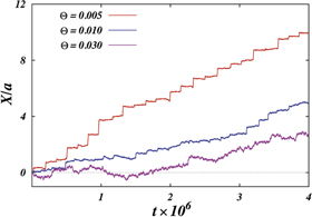
Figure 9. Displacement of the filament with time at three diferent temperatures; the data corresponds to about 50 cylces.
Download figure:
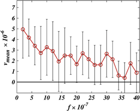
Standard image High-resolution imageWe have performed systematic long simulations, covering 300 motor cycles each at different temperatures and determined the corresponding mean filament velocities vmean. The results for the mean velocity vmean and its statistical dispersion at different temperatures are shown in figure 10.

Figure 10. Dependence of the mean filament velocity vmean on the dimensionless temperature Θ. Bars show statistical dispersion data. Averaging 300 cycles for each data point.
Download figure:
Standard image High-resolution imageFinally, figure 11 displays histograms of filament displacement per single cycle at the temperatures corresponding to different operation regimes. At relatively low temperature (figure 11(a)), almost all cycles result in the filament translation along the forward direction. There is however a large dispersion in step sizes. Occasional back steps in this regime are explained by Brownian motion of the filament during those parts of the cycle when the machine is detached from the filament. In the intermediate regime (figure 11(b)), a significant fraction of cycles results in the back steps, although the prevalence of forward steps is still clear. In the weak coupling regime (figure 11(c)), the distribution of steps is almost symmetric. Nonetheless, a slight bias towards the forward steps can still be observed, explaining the persistence of the directed filament motion.

Figure 11. Histograms of filament displacement per cycle at temperatures (a)  , (b)
, (b)  and
and  . Data for 1000 cycles is used.
Download figure:
Standard image High-resolution imageIn the above analysis, the rescaled temperature  has been varied in a broad interval to control the level of fluctuations in the system. While this variation may correspond to changes in the real temperature T, it can be also achieved by modifying the stiffness constant κ and thus making the EN more or less soft.
Operation under external load
Real protein motors are employed by biological cells not only to transport the load along the filaments, but also to generate force, as is indeed the case for muscle myosin. In the latter operation mode, the force generated by the motor counterbalances the external force, so that the net translational motion is absent. In this section, we investigate the operation of the proposed synthetic motor under the action of an external force.
Suppose that an external force fext is applied to the filament in the direction opposite to the direction of its motor-induced translational motion (see equation (21)). There are basically two effects of such external force. When the motor arm is attached to the filament, such a force will slow down the forward motion of the motor arm and the filament. In the other half of the cycle, when the arm is detached, this force induces a drift of the filament in the opposite direction.
Video 7 illustrates the motor operation in the presence of a strong external force, close to the stall condition, in the absence of thermal fluctuations. As can be observed, the motor pulls the attached filament in the forward direction for part of the cycle in the ligand-bound state. However, when the ligand is released and the motor arm moves away from the filament the attractive force between motor and filament decreases allowing the external force to dominate for a while and pushing the filament back.
When the external force is increased, the backward motion of the filament in the ligand-free state of the cycle becomes stronger. Under the stall condition, the active motor-induced forward motion of the filament should be on the average compensated by the force-induced backward motion. As a result, the net filament displacement will be vanishing.
By running simulations covering about 300 cycles each at different intensities of applied external force, we could determine the dependence of the mean filament velocity on the external force (see figure 12). As can be seen in figure 12, the mean propagation velocity of the filament indeed decreases and tends to zero, as the external force is increased. The stall condition could not be however reached in our simulations. The fluctuations in the propagation velocity were so rapidly increasing that extremely long simulations had to be performed to reliably identify the stall. Such long simulations were however beyond our capacity.
Figure 12. Dependence of the mean filament velocity on the external force. Bars show statistical dispersion of data; averaging has been done over 300 cycles for each data point. The dimensionless temperature is  .
.
Download figure:
Standard image High-resolution image
Methods
The final model, given by equations (17)–(21), is characterized by six dimensionless parameters  , c, μ, lc, fext and Θ. In our simulations, the first four parameters were kept fixed and had numerical values
  , c = 0.5, lc = 8.0 and
  . The temperature Θ has been varied. The values of the parameter fext are specified when simulations including external force have been performed.
The adjacency matrix for the machine  and the set
  of the equilibrium positions of the particles of the machine are given in the supplementary information. The natural lengths of the links connecting the ligand were
  .
.
The binding and release of ligand is governed by the specifying conditions on the hinge angle. If ϕ is in the interval ![$\phi \in [{\phi }_{0}-{{\rm{\Delta }}}_{0},{\phi }_{0}+{{\rm{\Delta }}}_{0}]$](https://content.cld.iop.org/journals/1367-2630/18/4/043006/revision1/njpaa1c2eieqn92.gif) , then binding of the ligand can take place with probability rate v0. On the other hand if ϕ is in the interval
, then binding of the ligand can take place with probability rate v0. On the other hand if ϕ is in the interval ![$\phi \in [{\phi }_{1}-{{\rm{\Delta }}}_{1},{\phi }_{1}+{{\rm{\Delta }}}_{1}]$](https://content.cld.iop.org/journals/1367-2630/18/4/043006/revision1/njpaa1c2eieqn93.gif) , then detachment of the ligand can take place with probability rate of v1. We do not allow dissociation of the ligand within the window
, then detachment of the ligand can take place with probability rate of v1. We do not allow dissociation of the ligand within the window ![$\phi \in [{\phi }_{0}-{{\rm{\Delta }}}_{0},{\phi }_{0}+{{\rm{\Delta }}}_{0}]$](https://content.cld.iop.org/journals/1367-2630/18/4/043006/revision1/njpaa1c2eieqn94.gif) . In our simulations the parameters we have used are the following:
. In our simulations the parameters we have used are the following:  ,
,  ,
,  and
and  . Further we assume that the product molecules are immediately removed from the reaction environment so that the back-binding of a product molecule once released is not possible.
We choose the coordinate system in such a way that its x-axis coincides with the filament. The machine was immobilized by fixing the positions of its 3 beads (i = 1, 2, 10) in this coordinate frame at  ,
,  and
and  . The filament could move along the x-axis and its position was characterized by the coordinate X(t) of the force centre n = 0.
The stochastic differential equations equations (17)–(21) were integrated with a first-order integration scheme with the fixed time step of 0.01. The initial conditions were prepared by taking the machine in its equilibrium configuration without the ligand, with the coordinates of all the beads given in the supplementary information. The initial position of the filament was  . The simulations were performed by using a standard quad-core PC and a single simulation covering 100 machine cycles took about 1 d to complete.
Discussion
There is a gap between two theoretical descriptions used to study protein motors—full MD and simple phenomenological approaches. Our study of a model system was intended to partially bridge this gap. The design of our synthetic motor model has been motivated by the operation of muscle myosin, but we have not attempted to mimic all principal aspects of myosin operation. The model is constructed in terms of ENs which have been also applied to describe myosin and other real molecular motors.
One arm of our synthetic motor is clamped to a rigid support much like muscle myosin (which is embedded in the thick filament of the muscle) while the other arm is free to swing back and forth similar to the motion of the myosin head. We have a passive filament in the model which imitates the role played by an actin filament. Our synthetic motor is powered by binding of a substrate, its conversion to a product and subsequent release of the product ligand. This is similar to the ATP binding at muscle myosin, the hydrolysis reaction and subsequent release of the products, i.e. of ADP and inorganic phosphate.
The myosin head grasps the actin filament during the power stroke in each operation cycle; this is achieved through ligand-induced conformational changes in the protein. Our model motor is not sophisticated enough to implement such additional conformational changes. Instead this aspect of motor operation is reproduced through the introduction of an attractive potential between the swinging arm and the filament. Such potential becomes effective only in one part of the cycle, when the arm moves closer and roughly parallel to the filament. Note that this model interaction mechanism is actually much less robust than active grasping; it requires exact positioning of the motor with respect to the filament; it would not also operate if the filament is flexible and its shape can fluctuate.
Because of the important differences, our model is only able to qualitatively emulate the operation of muscle myosin. It allows, however, to explore different possible operation regimes and elucidate the role of thermal fluctuations in this motor system.
In our simulations, dimensionless temperature was varied whereas the dimensional parameter , specifying the interaction between the motor and the filament, was kept constant. Since the aim of our study was to investigate the fluctuation effects, we have not taken into account possible temperature dependence of the model parameters, such as, e.g., the ligand binding and conversion rates. Three different operation regimes of the synthetic motor could be discerned, depending on the strength of thermal fluctuations.
The strong coupling was observed at a relatively low temperature. The interaction between the motor and filament was not then principally affected by thermal fluctuations and, in every cycle, the filament was getting transported forward by certain amount. This operation mode is therefore similar to that of a deterministic ratchet, with clear steps in each product conversion cycle. Note, however, that there is a broad distribution in the lengths of the filament steps and occasionally the steps in the back direction are already observed (see figure 11). Qualitatively, the strong coupling regime of our model motor is most closely resembling the myosin V operation [52].
The weak coupling regime was observed at a relatively high temperature, where the effects of thermal fluctuations on the filament dominate over its interactions with the motor. This regime can be compared to that of a Brownian ratchet. Because of high fluctuations, the motor arm cannot firmly hold in this case the filament within the power stroke part of the cycle and random sliding occurs. Nonetheless, the motor is still able, on the average, to transport the filament in the forward direction.
The intermittent regime is characterized by random alternation between the above two kinds of behaviour; it is observed in the intermediate range of temperatures.
Different stochastic ratchet models have been used in the past to model the behaviour of molecular motors. In such reduced models, the action of the motor is characterized by a single mechanical coordinate and a phenomenological ratchet potential is employed [36–41] and stationary flashing potentials have been used [53–55]. Travelling flashing periodic potentials have been considered in describing polymer dynamics [56]. Our model is most close to a ratchet with the travelling flashing potential. During the power stroke, the motor arm approaches the filament and moves forward along it. It interacts attractively with the force centres periodically placed along the filament, so that a periodic travelling potential acting on the filament is created. However, in contrast to what is usually assumed in the ratchet models, interactions with the filament are also influencing the motion of the motor arm. Therefore, the flashing travelling potential in our motor system is not externally imposed, but rather results from the consistent internal operation of the entire system. As will be shown in a separate publication, the considered synthetic motor can be approximately described by a reduced stochastic ratchet model with two mechanical coordinates.
While special attention has been paid in this study to make the constructed model motor similar in its structure and operation to real protein motors, several simplifying assumptions have been made. Particularly, we have assumed that, once bound, the substrate cannot dissociate from the motor without undergoing conversion to the product ligand. Hence, substrate affinity was assumed to be high. Furthermore, reverse binding of the product to the motor—and possible back conversion cycles of products to substrates—were not allowed. This corresponds to an assumption that the products are immediately evacuated once they are released. Both such assumptions can be however lifted. The operation of the model motor under fully reversible conditions will be a subject of a separate publication, where the energetic efficiency aspects will also be carefully discussed.
In our study, the questions of physical implementation of the hypothetical synthetic motor were not addressed. We did not specify any concrete molecular system which would be able to operate in the proposed way. Although the considered EN is similar to the ENs of actual proteins, we cannot outline any polypeptide chain which would fold into the respective conformation. Construction of amino acid chains folding into required conformations represents a challenging problem of protein engineering. Probably, the first physically implemented synthetic protein motors would be obtained by purposeful modification of already existing molecular structures, rather than by the design of completely new ones. The results of our investigations may help to elucidate the constraints and design principles when the actual motor construction is undertaken in the future. They can also contribute to better understanding of how the known biological protein motors work.
Acknowledgments
The authors thank R D Astumian and Y Togashi for stimulating discussions. Financial support from the Volkswagen Foundation (Germany) within the project 'Self-organizing networks of interacting machines; Principles of design, control and functional optimization' is gratefully acknowledged.
Supplementary data. (5 MB, txt) fil_pos.txt: Initial position of the power centres on the filament.
Movie 1. (2.6 MB, mp4) Cyclic operation of the machine, in the absence of noise.
Movie 3. (1.3 MB, mp4) Motor operation at low temperatures in absence of substrate conversion.
Movie 4. (2.0 MB, mp4) Motor operation at higher temperatures in absence of substrate conversion.