


Abstract
We propose a new type of traveling wave pattern, one that can adapt to the size of physical system in which it is embedded. Such a system arises when the initial state has an instability for a range of wavevectors, k, that extends down to k = 0, connecting at that point to two symmetry modes of the underlying dynamical system. The Min system of proteins in E. coli is such a system with the symmetry emerging from the global conservation of two proteins, MinD and MinE. For this and related systems, traveling waves can adiabatically deform as the system is increased in size without the increase in node number that would be expected for an oscillatory version of a Turing instability containing an allowed wavenumber band with a finite minimum.
Export citation and abstract BibTeX RIS
One of the ways in which a non-equilibrium system can lead to pattern formation is via a traveling wave bifurcation [1]. In such a system, the uniform state becomes unstable to modes at a finite wave vector k and a finite frequency ω leading to a variety of phenomena involving nonlinear traveling wave states. This scenario has proven relevant for processes ranging from binary fluid convection [2, 3] to electro-hydrodynamics in liquid crystals [4] to the sloshing of Min proteins in bacteria [5–14].
To date, this instability has been viewed as an oscillatory analog of the familiar Turing instability. Such an analogy implies that as a function of some control parameter, the instability sets in at a critical threshold value of the parameter at some given  . Furthermore, above threshold, there is a band of unstable wavevectors stretching from
  . Here we show that there exists a previously unconsidered possibility, namely that for some systems with a particular symmetry, kmin equals zero. This dramatically changes the nature of the nonlinear patterns that form, as there is no predetermined length scale for the emergent structure; instead, the waves are able to self-adapt to the size of the physical system. As we will discuss, this is the traveling wave analog of what happens in viscous fingering [15, 16] where the static bifurcation extends to
  . Models for the aforementioned Min dynamics offer a specific realization of this new paradigm. Moreover, the self-adaptation provides a mechanism whereby the dynamical pattern can maintain a one node form as the cell expands during growth.
We start with the model of [11, 17] for the Min system. There are two proteins, MinD and MinE, each of which can be on the membrane (m) or in the cytosol (c). The two proteins can reversibly desorb and adsorb, and adsorption of MinE involves it directly binding to an already membrane resident MinD. Additional nonlinearities emerge from the assumed cooperativity in the desorption rates. Adding in diffusion in the compartments leads in one spatial dimensions to the 4 coupled pde's


where cD and cE are the cytosol concentrations of MinD and MinE, cd is the concentration of MinD on the membrane and cde is the concentration of the MinD/MinE complex on the membrane and the rates are

Of critical importance to the physics of this system are two features. First, the diffusion constants of the membrane-bound species are orders of magnitude smaller than their values for the same protein in the cytosol. We will see that this property will guarantee the existence of an instability which drives the pattern formation and also will enable a simplification of the dynamics, at least for small system size. Second, the model contains two global conservation laws; the total number of both MinD and MinE proteins in the system are unchanged by each of the reactions, so that they are determined solely by the initial conditions. To see what this implies, we imagine we have found a uniform steady-state solution of the model and calculate the fate of a small perturbation around this solution, so that
with analogous expressions for the other concentrations. This leads in a standard manner to a 4 × 4 homogeneous linear system, with the growth rates Ω being given by the eigenvalues of the k-dependent stability matrix. The results of such a calculation for the most unstable mode, where for the moment we ignore the quantization of k induced by the boundaries, are presented in figure 1. We see that for  , there is a complex unstable mode, whose (complex) growth rate goes to 0 in the limit
  . We shall now show that this is a direct result of the global conservation laws. At k = 0, due to these laws, the sums of equations 1(a, b, d) and equations 1(b, d) are identically zero, as shifts in the overall levels of either the conserved MinD or MinE proteins due to the perturbation are left unchanged by the dynamics. Hence
  is a doubly degenerate eigenvalue for k = 0, with left eigenvectors
  and
and  . We can then calculate the shift in
  for these two modes for small k using what amounts to degenerate perturbation theory in quantum mechanics, generalized to non-Hermitian matrices. To leading order, we computing the projection of the perturbation, i.e., the diffusion terms in the stability matrix, namely
  onto the basis of the degenerate
  subspace to obtain the reduced stability matrix

where the  are the corresponding right eigenvectors of the two k = 0 zero modes, which satisfy the orthonomality condition
  . We then have to diagonalize
  to find
  . For the parameter set used in [11], the steady-state is
  ,
,  ,
,  ,
,  and this gives rise to
for pair-wise equal cytosol (Dc) and membrane (Dm) diffusivities. This matrix always has a pair of complex eigenvalues, as

This complex pair is unstable as long as

which is easily satisfied by the biophysical parameters, as we saw in figure 1. In general, the initial rise of  with k depends on the relatively large cytosol diffusion constants whereas the value of k at which the system restabilizes depends on the small membranal ones. In the limit of very large diffusion constant ratio between the cytosol and membranal fields and for equal membranal diffusivities, Dm, the spectrum approaches (for k strictly non-zero) the simple form
  for complex
  with a positive real part.
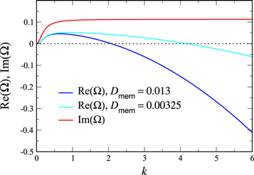
Figure 1. The growth rate  and frequency
  of the most unstable mode of the linear stability operator constructed about the uniform steady-state solution, for two different values of the diffusion rate, Dm, of the two membrane-bound species,
  . The frequencies for the two cases are indistinguishable at the resolution of the graph. The other parameters, as taken from ([11]), are:
  ,
,  ,
,  ,
,  ,
,  ,
,  ,
,  ,
,  . In the following, all lengths with be in
  and times in
  and explicit units will be dropped.
Download figure:
Standard image High-resolution imageThis stability structure presents a new twist on what happens in pattern forming systems such as viscous fingering and dendritic crystal growth [15, 16]. There, translation invariance of the base system guarantees a single zero k = 0 eigenvalue which gives rise to a real-mode instability for  . A related idea has arisen in the context of cellular processes that have one chemical component being exchanged between different compartments but is globally conserved [18]. In our system the existence of two zero modes and of course the non-symmetric nature of the stability matrix allows for a pair of complex conjugate modes to have a positive growth rate. The study of those interfacial systems has revealed characteristic differences between the nonlinear states that emerge as compared to those in related systems such as directional solidification [19] which have a regular Turing-like mode spectrum. Here the basic pattern is the traveling wave, which due to the instability extending down to k = 0, should exist up to very large wavelengths. There are thus two new features here, compared to the standard Turing case. One is the fact that the basic unstable mode is a traveling wave as opposed to a stationary spatial oscillation. It is in general quite hard to arrange parameters such as to guarantee that the basic instability is a traveling wave, while preventing a k = 0 Hopf temporally oscillating mode. Here however the marginality of the k = 0 modes makes the travellng wave instability very natural, as a k = 0 Hopf instability is impossible. Further, the standard Turing instability has a narrow band of allowed wavelengths, at least close to threshold, while here the instability extends to infinite wavelength.
It is possible to show that the traveling wave pattern arises as a supercritical bifurcation as L is increased past  , so that the unstable mode is an allowed wavevector. Thus the amplitude grows as
  as the system size is increased. For larger systems, we must turn to a numerical study of our traveling wave pattern. In the top panel of figure 2, we show an example of a traveling wave solution, corresponding to the parameter set already used above, for a periodic system of size
  . The second takes the limit of infinite diffusivity for the cytosolic species cD and cE; for the latter case, the model is globally coupled with the value of these fields determined at all times by the integral constraints
For this size system, which is not much larger than the minimal size for the instability,  , this traveling wave pattern appears to be the unique attractor of the system, arising from generic initial conditions.
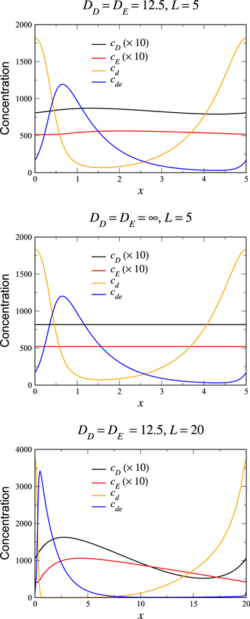
Figure 2. The uniformly leftward propagating wave solution, with  . Top: the solution for the parameters of [11], for which the stability analysis is shown in figure 1 (blue curve). The length of the periodic system is L = 5. Middle: the solution for the limit
  , with all other parameters as above. The membranal field profiles are basically unchanged from the above graph. Bottom: the solution for the same parameters as in the top panel, for the larger system L = 20. The peak in the membranal fields is roughly the same width as in the top panel, so that L-scaled coordinates, it appears much sharper. Away from the peak the solutal fields appear similar to the top panel, indicating that these features scale linearly with L. The variation of the solutal fields is much increased over that of the top panel.
Download figure:
Standard image High-resolution imageThe solution can thus be generated by running a simulation and waiting for the system to settle into this uniformly propagating state, which perforce must be linearly stable. Alternatively, we can directly solve the steady-state equations in the moving frame of reference, so that the fields are only functions of x − vt and the equations become ordinary differential equations, by an iterative scheme acting upon the field values at collocation points. Since there are 4 second-order equations, we have to impose eight conditions. Six of these are the continuity of the four fields and two of the derivative fields across x = L. Two are the global constraints on the DT and ET. Because of translation invariance we can arbitrarily choose one of the fields to have a known value at say  and reduce the number of unknowns by one. Then the number of equations to be solved is one greater than the field unknowns, necessitating the use of the velocity as the final unknown. One can check that we get the same results from both of these methods. The second approach is specifically convenient if one has a solution for some parameter set and wishes to find a solution at a nearby one, as in that case there is a very good initial guess with which to start the iteration. We can see from these graphs that there is nothing singular about the infinite-Dc global limit at least as far as this type of solution is concerned.
We see that while the cytosol concentrations are relatively featureless (exactly so in the globally coupled,  , limit), the membranal fields each have a single peak, located close to each other. As we take L larger, as in the bottom plot of figure 2, this structure is maintained, with the peaks having roughly the same width, and so occupying a smaller fraction of the system. The system settles into a scaling form of the solution in which the pattern consists of two parts. There is an inner region, which for the bottom frame of figure 2 lies at around the origin which gets thinner (in rescaled coordinates) as L increases. The rest of the box has an 'outer' solution which scales linearly with L. The velocity of the solution scales as L once the system is in the scaling regime, which for our parameters occurs for
  . It is interesting to note that the large cytosol diffusion is much less successful in eliminating the variation in the cytosol fields in the larger L system.
We can understand this solution by looking separately at the two aforementioned regions, in the globally coupled limit, keeping cD and cE (as opposed to DT and ET; in the globally coupled limit, this is just a different path in parameter space, which happens to exhibit less L dependence) fixed as we increase L. We assume a dependence only on  and hence the time derivatives become
  . In the outer region, the slow diffusion is irrelevant and the only spatial derivative is the velocity term. Thus, having
  (as can be verified from the numerical solutions) immediately allows the outer solution to have spatial decays away from the peak which become L independent in the rescaled coordinate. In the inner region, we have in general three terms that are important; the velocity term, the diffusion term and the cubic term that occurs (with opposite sign) in both the cd and cde equations. In fact, if we add the two equations and assume equal diffusivities, we get that
  does not have any driving term and one can easily check from the numerical solution that it is approximately constant on the inner scale, which is the original L independent length scale. Let us denote by A the constant value of this sum at the location of the inner zone. The numerics indicates that this quantity also scales linearly with L. If we rescale lengths by
  , velocity by
  , and membranal concentrations by L as well, (
 , etc) we get the equations
This pair of conjugate equations are familiar from the literature on pattern formation, in the context of front solutions in bistable systems such as the Ginzburg–Landau equation. We can define a 'potential' function  to recast the equation for
  , e.g. as that of a 'particle' moving with damping
  in a potential well,
where the potential is obviously

This potential has a maximum at cd = 0 and, interestingly, a point of inflection at  . Since there is no minimum, for small dampling a particle starting at cd = 0 at
  will escape to infinite cd. Above a critical damping, the particle approaches the point of inflection as a power-law in time, since the force is quadratic in the distance to this point. The critical damping is equal to
  , for which the approach to the point of inflection is exponential in time, as can be seen be directly substituting in the ansatz
  for some width w. Thus, an inner solution exists for all velocities greater that
  . If we call this solution
  , we have the final forms
  and
and  . There are two unknowns, namely
  and the scaled velocity
  .
.
The construction is then completed by integrating the L-independent outer equations in the variable z, where as mentioned above diffusion is ignored. One can then integrate the coupled first-order outer equations starting immediately past zinner with the initial conditions  ,
,  and demand that the solution at
  returns back to the inner solution left asymptote
  ,
,  . These conditions determine the two unknowns. The fact that the system supports a scale-invariant nonlinear traveling wave is, we believe, traceable to the nature of the original stability; the system can use its ability to self-amplify at any non-zero k to form this solution.
While this 'single pulse' wave appears to be the unique stable steady-state solution for relatively small L, as L increases this ceases to be the case. One way to see this is to start with an initial condition which is composed of two  pulses. For
  , for our 'standard' parameters, the two peak solution develops an instability and eventually reaches the single pulse solution appropriate to a system size of L. This process is demonstrated in figure 3 for L = 20. This is analogous to what was established long ago for a periodic array of Saffman–Taylor fingers [20]. But, here, the full story is complicated and in general we find three regions for the asymptotic state arising from these conditions. For
  , we obtain full coarsening as above. At larger L the two pulse pattern is stable, coexisting with the stable one pulse wave. The onset of the instability as L decreases below Lc1 is a (apparently subcritical) Hopf bifurcation. At even larger L, there is a supercritical pitchfork bifurcation to a non-symmetric two pulse state. Analogously, one can start with a three pulse initial condition in a
  box and find regions of stable non-symmetric solutions at large enough L. In addition, the larger range of unstable wavevectors at increasing L appears to result in a shrinking of the basin of attraction of these steady-state solutions; this remains to be quantitatively analyzed. It should also be noted that, for finite solute diffusion, the single pulse solution ceases to exist beyond some maximal L. When this occurs, the only traveling wave state will have multiple peaks.
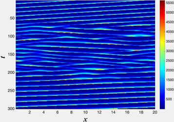
Figure 3. The merging of a two peak traveling wave composed of two L = 10 solutions into a single L = 20 steady traveling wave. The cd field is presented, the cde field would look very similar. The parameters are the same as in the top panel of figure 2.
Download figure:
Standard image High-resolution imageBecause of the stability of the single pulse solution, the system will stay in this state as the box size is adiabatically increased. To see this, we assume that the system is regulated so as to maintain a fixed overall average concentration of MinD and MinE and insert more of these proteins uniformly into the cytoplasm as we expand the cell. Following [21], the system equations then read

where  is the time-dependent length of the system and
  is the scaled spatial coordinate. Figure 4 shows clearly that the one pulse wave will maintain its global topology for a very large range of scales.

Figure 4. The pattern produced by an exponentially growing system, with doubling time of 30 min and initial size of L = 4. Solutal MinD, MinE is added to keep the overall average MinD and MinE concentrations fixed. The membranal field cd is displayed, cde looks very similar. The system quickly settles into a single pulse traveling wave solution and preserves this form, despite the continually change in L. The increase in amplitude and initial increase in temporal period are apparent. The other parameters are the same as in the top panel of figure 2.
Download figure:
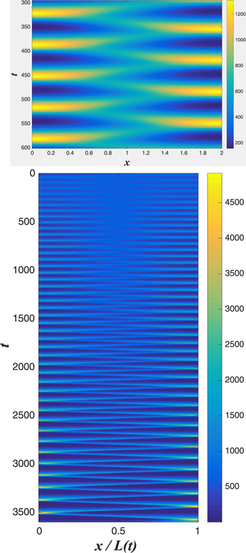
Standard image High-resolution imageOf course, the actual Min system does not live in a periodic domain; even if one adopts the simplification of ignoring the actual compartment structure of the cell into membrane and cytosol in favor of a bi-continuous approach (as is done here), one should obviously use zero flux conditions at the cell edges. So, it is useful to ask about the from of the nonlinear traveling wave state to the dynamics in a fixed box. In the top panel of figure 5, we present snapshots of simulations for small cells, showing clearly a 'sloshing' wave pattern with sharply decreased amplitude at the cell center. Most importantly this topology is not changed as the cell expands, even as the pattern becomes more like a traveling wave bouncing back and forth (see the bottom panel of figure 5). The time-average concentrations maintain a single node at the center even as the cell doubles; this is necessary for the functional role of the Min system in defining the precise midpoint of the cell [12, 22]. The self-adjustment property of the system allows this to take place without any fine-tuning of system parameters.
Figure 5. Top: a 'sloshing' pattern produced in an L = 2 with reflecting boundary conditions. One sees that the amplitude is concentrated near the edges and the amplitude is minimal at the center. A disturbance appears on the left, waxes and wanes 180° out of phase with the disturbance on the left. Bottom: the adiabatic adjustment of the above 'sloshing' pattern in an exponentially growing system, with a doubling time of 30 min and an initial size L = 1.5. Initially, when the system is small, the system quickly settles into the sloshing pattern seen above, with an amplitude minimum in the center. Later, when the system is larger, the pattern more closely resembles the one-pulse traveling wave solution bouncing between the walls. The other parameters are the same as in the top panel of figure 2.
Download figure:
Standard image High-resolution image
It is critical to realize that very few of our findings should have anything to do with the detailed assumptions of the model. For example, if one uses more recent and presumably more realistic models for Min dynamics proposed in [10, 23], the existence of two conservation laws will again guarantee that the wave instability will extend down to k = 0 and therefore we can predict the existence of self-adjusting traveling wave states. This of course needs to be investigated in detail. A more uncertain situation holds for a recently studied case of a  wave instability arising during the frictional sliding of one surface above a second [24]. Here the fact that the base state with uniform sliding is explicitly not reflection symmetric and hence there need not be modes at both
  and
and  at the same complex value of Ω; in other words, there is a preferred direction of wave propagation and this one unstable wave can be connected to just one symmetry mode as
  . The extent to which this difference matters for the nonlinear state remains to be studied. We also expect the general features explored here will persist in a full two-dimensional model where the 2-d nature of the cytosol is treated explicitly [17].
Acknowledgments
This work was supported by the US National Science Foundation Physics Frontier Center program grant no. PHY-1427654, the National Science Foundation Molecular and Cellular Biology (MCB) Division Grant MCB-1241332 and the US-Israel Binational Science Foundation Grant no. 2015619. We gratefully acknowledge the hospitality of the Aspen Center for Physics, where this work was started.