


Abstract
A resistivity model for non-crystalline, solid-density carbon and hydrocarbons is presented for such materials heated by short-pulse, ultra-intense lasers. Electron-impact excitation of C atoms and ions was included in this model, and calculation of resistivity curves with and without accounting for excitations indicates that excitations contribute >50% of the resistivity in the 3–20 eV range. This implies that electron-impact excitations make a similar contribution to electron–ion scattering, and thus models not accounting for electron-impact excitation may underestimate the resistivity of dense plasmas in this temperature range.
Export citation and abstract BibTeX RIS

Content from this work may be used under the terms of the Creative Commons Attribution 3.0 licence. Any further distribution of this work must maintain attribution to the author(s) and the title of the work, journal citation and DOI.
1. Introduction
The electrical resistivity of dense matter has been a problem of considerable importance for condensed matter and solid state physics, plasma physics, as well as astrophysics and geophysics. The development of new technologies (such as chirped pulse amplification lasers) has introduced new methods for generating matter at high densities and temperatures, thus expanding the range of conditions over which electrical conductivity calculations might be compared to experiment and has thus blurred previous distinctions between different disciplines of physics.
When ultra-intense lasers (>1018 Wcm−2) irradiate dense plasmas, a characteristic feature of the interaction is the generation of a high current density spray of relativistic (or 'fast') electrons [1–9]. At such high current densities (>1015 Am−2) and MeV energies, the fast electron dynamics is not dominated by collisions with the background electrons and ions, but is instead dominated by the resistively generated electric and magnetic fields [10–12]. Since these are resistively generated fields, the resistivity of solid density plasmas in the temperature range of 1–100 eV (and even above this) is of great interest to researchers studying the propagation of laser-generated fast electrons in dense plasmas. The fast electrons are responsible for a number of important secondary processes in ultra-intense laser-solid interactions that are of interest for their potential applications [13]. These include x-ray generation [3], proton and ion acceleration [14, 15], and possibly nuclear reactions via the generation of gamma-rays [16]. Fast electron transport through solid targets is a process that affects all of these potential applications, and thus the understanding of electrical resistivity across a wide range of conditions may play an important role in the realization of these applications.
At very high background temperatures (≈1 keV and higher), one might argue that the situation is simpler, at least in relative terms, as the background plasma is then closer to being a classical, fully ionized plasma (assuming that Z is not very high) with the resistivity determined by the Spitzer resistivity [17]. Irrespective of whether or not this is a good argument, since these solid targets start out at ambient temperature, they are effectively cold at the start of the interaction, so one cannot avoid having to consider the resistivity at solid density at temperatures at which the material might be considered a form of warm dense matter (WDM), e.g. 1–10 eV, or even in the solid-state/condense matter regime (<1 eV). This is a much more difficult situation to consider, however certain experiments present a clear case for this 'low' temperature regime defining the nature of the resulting transport pattern [18]. Thus the resistivity issue spans a number of different regimes that are often the concern of separate disciplines.
One approach is to use density functional quantum molecular dynamics (DF-QMDs) to determine the resistivity at a given temperature and density. This method has been applied successfully to problems in WDM such as the ion–ion structure factor in warm dense Al [19, 20], and it was used to obtain resistivities at low temperatures in [18]. While the method is very powerful, there are three problems with solely using DF-QMD to obtain resistivity curves : (i) all fundamental simulation methods, including many in plasma physics, and especially DF-QMD, require interpretation. Interpretation requires some sort of complementary theoretical framework other than just DF-QMD calculations. (ii) It can be very time consuming and dependent on access to significant computational resources to build resistivity curves using a series of DF-QMD calculations. (iii) Simulation codes that use these resistivity curves (e.g., see hybrid codes in [5, 10, 18, 21–23]) would ideally like to make use of a simpler model that is easy to implement, executes quickly, but can cope with a wide range of different parameters. Previously, the third issue has driven plasma physicists interested in high energy density systems to develop wide-ranging (albeit approximate) resistivity models such as that of Lee and More [24, 25].
In this paper, we report on the development of a resistivity model for non-crystalline carbon, with a focus on treating relatively low temperatures, especially the 5–30 eV range. In principle the model is extendible to other materials provided that suitable cross-sections are available. In the context of the present work, non-crystalline carbon was chosen for the following reasons : (i) it was the subject of study in previous work [18] and DF-QMD calculations were used to generate a resistivity curve for this material in that study, (ii) plastics and other organic compounds are standard targets in the field of laser–plasma interactions and fast electron transport studies, so the resistivity of systems based around disordered carbon is highly important to this research community. We believe that the model can be integrated into existing plasma simulation codes relatively easily, if required.
The results of our resistivity model are compared to the results previously obtained using DF-QMD calculations. It was found that, in the important 5–30 eV region, electron–ion collisions only account for less than half of the resistivity. Remarkably, for some temperatures, the difference between the DF-QMD calculation and a resistivity model based on e–i, e–e, and e–n scattering is a factor of 4–5. This shows that there is substantial and very much non-incremental progress yet to be made in understanding resistivity in this regime. Futhermore, this observation suggested that inelastic collision processes in the partially ionized dense carbon plasma were more important. Both electron-impact excitation and electron-impact ionization were considered, and it was found that electron-impact excitation processes dominate the resistivity in the 5–30 eV range. It is likely that accounting for electron-impact excitations will significantly affect the calculated resistivity for a wide range of non-crystalline materials. As the inclusion of excitations leads to an increase in resistivity by a factor of 2–3 in this temperature range, this can have a very significant effect on both fast electron transport and the interpretation of laser-solid experiments.
For the sake of clarity : note that in this paper we use the term 'electron–ion' collisions in the sense that it is normally used in plasma physics, that is to refer only to elastic scattering of electrons from ions and not to any inelastic processes.
2. Resistivity model
The resistivity model that we have developed is based on the following assumptions : (i) the free electron population is treated as a uniform electron gas of arbitrary degeneracy (i.e., a 'jellium' approximation), (ii) the ions are assumed to be highly disordered (i.e., a 'randium' approximation). The assumption of no short or long range order is, of course, consistent with our aim of stuyding the resistivity of non-crystalline materials. However it has significant consequences for how the model should be constructed. As has been observed for liquid metals [26], the lack of any long range ordering of the ions, implies that bound electrons will be in localized atomic-like states as opposed to the band structure situation that would occur in a fully crystalline material. Similarly this means that there are no coherence effects when conduction electrons scatter from ions, so, unlike the crystalline situation, electron–ion scattering does not cancel out. The electrostatic screening length in this system is calculated using Lindhard theory [27] throughout.
The resistivity model that we have developed is based on the relaxation time approximation [28]. In this relaxation time approximation the electron distribution function can be written as

where momentum space is described in terms of spherical polar coordinates with θ being the polar angle, and p being the magnitude of momentum. The term, f0, describes the isotropic part of the distribution function, and f1 describes the anisotropy induced by the electric field. On substituting this into the kinetic equation, one then arrives at the following for the perturbation to equilbrium

where E is the electric field, and  is the collision time for an electron with momentum p. In order to relate this to resistivity, the first moment is taken to determine the current density, j. After integrating over the azimuthal and polar angular coordinates in momentum space, one obtains

and substituting in equation (2) yields

From the definition of resistivity ( , where η is the resistivity) one finally obtains the main expression for the resistivity in the relaxation time approximation

Since one aims to handle arbitrary degeneracy, f0 will be a Fermi–Dirac distribution. What remains is to determine the collision times for each collision process (electron–ion, electron–neutral, electron-impact excitation of ions and atoms, etc). A single collision time is obtained from all of these via

where  is the collision time of the kth process. In addition to this there must be an ionization model to determine the electron density (or
  , the effective ion charge). Many resistivity models use the Thomas–Fermi model, however this is prone to predicting too high an ionization level in low temperature solid density plasmas. To avoid this we have used Desjarlais' modification to the Thomas–Fermi model [25]. In the subsequent sub-sections we describe how
  is determined for each separate collision process.
2.1. Electron–ion collisions
For the electron–ion collisions we have made use of the approach to scattering via the quantum Lenard–Balescu (QLB) equation [29]. For a dynamically screened Couloumb potential this results in the e–i collision time being given by

where ni is the ion density, k is the electron wavenumber ( ), and
  is the screening wavenumber and is related to the screening length, ls, via
  . This expression can be evaluated analytically (e.g., by means of substituting a hyperbolic function), to yield

where  . This is a distinctly different approach from the standard Lee–More model [24] which uses a Landau–Spitzer (LS) approach which results in one obtaining Coulomb logarithms which need to be artificially capped. The QLB approach has also been used to address the problem of electron–ion equilibriation in WDM [30, 31].
2.2. Electron–electron collisions
In order to account for the effect of electron–electron collisions we have used the approach described by Ebeling and co-workers [32], in which the e–i collision time is reduced by a certain factor. The reduction factor is calculated as follows. First we define a reduction factor in the non-degenerate limit,  , using the results of Van Odenhoven and Schram [33]

and we then re-scale this according to the prescription of Bespalov and Polishchuk [34] to account for degeneracy

where TF is the Fermi temperature, and T is the temperature. The e–i collision time is then multiplied by this factor.
2.3. Electron–neutral scattering
At low temperatures it is possible that  i.e. not all atoms have undergone the first ionization. This means that we must account for the elastic scattering of electrons from neutral carbon atoms. At any given energy we obtain a cross-section for e–n scattering from Desjarlais' fit [25] to a cross-section that is calculated in the Born approximation using screened potentials [35, 36]. Below we give the expression used from Desjarlais [25]

where all lengths are in units of aB (the Bohr radius),  is the dipole polarizability (in units of aB3), k is the wavenumber of the incident electron, and
 ![${r}_{0}=\sqrt[4]{{\alpha }_{D}{a}_{B}/2{Z}^{1/3}}$](https://content.cld.iop.org/journals/1367-2630/17/8/083045/revision1/njp517816ieqn13.gif) is a cut-off radius. The coefficients in the denominator are given by
is a cut-off radius. The coefficients in the denominator are given by


The cross-section that this is a fit to is itself obtained using the 'polarization potential' [35, 36]. This is a model potential [37] that has often been used for electron–neutral scattering, of the general form  . At large radii this potential corresponds to a dipolar potential, as one would physically expect. In the polarized atom the potential is not singular at the origin, and the cut-off, r0 ensures that this does not occur in the model potential. The dipole polarizability used for neutral carbon atoms was taken to be
  based on the results of Miller and Kelly [38]. Once the cross section has been obtained the electron–neutral scattering time is determined from

where nC is the number density of neutral carbon atoms, and ve is the electron velocity magnitude.
2.4. Electron-impact excitation
At moderately low temperatures the partially ionized state of warm dense carbon means that electrons can collide with atomic states of multi-electron carbon ions inelastically resulting in electrons being promoted to excited states. This is contingent on the 'randium' assumption for the carbon ions (that they are highly disordered), as only in this case is the assumption of localized atomic-like states a good one [26]. Having assumed this, we then take the cross-sections for electron-impact excitation from Itikawa et al's [39] compilation of electron-impact excitation cross-sections for isolated carbon atoms. These will neglect any effects of being immersed in dense plasmas, so the effect of this on the cross-sections is neglected. Excitation processes were only considered for C+–C3+ as the excitation energies for the highest ionization states is so large as to have negligible effect on the resistivity. The population of the electronic states was determined from the Boltzmann distribution and the ion density obtained from the ionization model.
In the case of  we only considered the 2s2S and 2p 2P states and electron impact excitation from the former to the latter. The energy for this transition is 8 eV. The next transition is the 2p 2P to 3 s 2S transition with an energy of 29.55 eV. This excitation was found to be negligible so this and all other possible electronic excitations were neglected.
For  we considered the excitations from the 2s2 1S to the 2s2p1P state and the excitation from the 2s2p 3P to the 2p2 3P state. The former excitation has an energy of 12.69 eV and the latter has an energy of 10.54 eV. The cross-section for excitation from the 2s2 1S to the 2s2p 3P state (energy of 6.5 eV) is sufficiently small for this to play a negligible role.
For C+ we considered the following transitions : 2s22p 2P to 2s2p2 2D, 2s22p 2P to 2s2p2 2P, 2 s22p 2P to 2s2p2 4P, 2s2p2 4P to 2s2p2 2D, 2s2p2 2D to 2s2p2 2S, 2s2p2 2D to 2s2p2 2P, 2s2p2 4P to 2s2p2 2S, and 2s2p2 4P to 2s2p2 2P. The energies relative to the ground state (2s22p 2P) are : 5.33 eV (2s2p2 4P), 9.29 eV (2s2p2 2D), 11.96 eV (2s2p2 2S), and 13.71 eV (2s2p2 2P).
The excitation time for each excitation at a given electron momentum was then determined via  , where n is the density of carbon atoms in the initial state of the excitation process.
2.5. Electron-impact ionization
Electron impact ionization can potentially also affect the resistivity. In order to examine the significance of electron impact ionization we included it by estimating the cross section from the Lotz formula [40]

where  is the incident electron energy in eV, UZ is the ionization energy in eV (from the Zth ionization state), and is the number of equivalent electron in the shell from which the ionization occurs. In order to account for continuum lowering, the ionization energy is reduced by
  , where we use the approximation

where  is the inter-ionic distance, this being the simplest estimate of the continuum lowering [2]. Note that the inter-ionic distance is obtained from
 ![${r}_{ii}=\sqrt[3]{3/4\pi {n}_{i}}$](https://content.cld.iop.org/journals/1367-2630/17/8/083045/revision1/njp517816ieqn21.gif) , and for vitreous carbon is 0.147 nm. The electron impact ionization time is then determined via
, and for vitreous carbon is 0.147 nm. The electron impact ionization time is then determined via  . We have assessed the role of electron impact ionization under both the assumption that all ions are in the ground electronic state, and for a Boltzmann distribution that includes both the ground state and the first excited state. In both cases we found that ionization processes made only a very minor contribution to the resistivity. We therefore did not include electron-impact ionization in the final model.
3. Results
In this section we present resistivity curves that have been calculated using the resistivity model described in the previous section. For the case of vitreous carbon we compare this to results obtained from DF-QMD calculations in a previous study [18].
3.1. Vitreous carbon
We have calculated a resistivity curve for vitreous, or glassy, carbon assuming a density of  kg m−3. The results for the full model is plotted in figure 1.

Figure 1. Plot of resistivity curve for vitreous carbon at 1500 kg m−3 as calculated by the full model against results from DF-QMD calculations. Also shown are the resistivity curves that are calculated when only e–i and e–e scattering are included, and when only e–i,e–e and e–n scattering are included.
Download figure:
Standard image High-resolution imageThese results are plotted against results from DF-QMD calculations, and against a curve calculated when only electron–ion and electron–electron scattering are included, as well as a curve calculated when only electron–ion, electron–electron, and electron–neutral scattering are included. This plot shows that the resistivity obtained from the DF-QMD calculation in the 2–20 eV range is much higher than the resistivity that is calculated when only e–i, e–e and e–n scattering is accounted for by more than a factor of 4. The plot shows that when we attempt to account for the effects of electron-impact excitation the resistivity curve that we obtain is much closer (albeit still not in perfect agreement) to the resistivity obtained from the DF-QMD calculation.
The comparison between the model with and without excitation can be done more quantitatively by calculating the percentage of the resistivity due to excitation (according to the model) from the resistivity curves obtained with and without excitation. The results of this calculation are shown in figure 2.
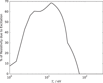
Figure 2. Plot of the fraction (as a percentage) of the resistivity in the full model that is due to excitation process against electron temperature.
Download figure:
Standard image High-resolution imageFrom figure 2 we find that in the 2–20 eV range, excitation processes account for over 50% of the resistivity, and this is up to 70% at some points. It is therefore clear that excitation is at least as equally important as standard scattering processes in this temperature range (for solid vitreous carbon), and in some cases excitation process make the dominant contribution to the resistivity.
In addition to the contribution of the excitation processes, we also find, however, that the resistivity model seems to over-predict the resistivity at very low temperatures compared to the DF-QMD calculation. There could be a number of reasons for this, which stem from the present model not treating the solid-state regime well, for example : in the solid state, both amorphous and glassy carbon are better characterized as poor conductors rather than poor insulators. The conduction mechanism has been described as a hopping mechanism between localized states. Such a mechanism is not described by this model, so it is not entirely surprising that the present model is deficient at very low temperatures.
Of course, one could question whether the use of the QLB approach, as opposed to other approaches, has lead us to significantly underestimate the e–i collision time and thus its contribution to the resistivity. To address this question we start by noting that we could instead follow the LS approach in this model by adopting the following expression for the e–i collision time:

instead of equation (7). This is very much like the e–i scattering time used by the model of Lee and More. However we must choose values for the arbitrary cut-offs, and for this we will follow Lee and More by taking kmin to be the inverse screening length, but we keep  . In figure 3 we show the resistivity due to the e–i collisions alone as calculated by the QLB and LS approaches (the version we described above). Figure 3 shows that reverting to the LS approach leads to an increase in the contribution to the resistivity due to e–i collisions compared to the QLB approach. Of course, one can question how physical this is [30, 31], and whether it is correct to believe the LS approach merely because it predicts a higher resistivity. However when we compare both results to the DF-QMD simulation results we see that the difference in the e–i contributions from either approach are small in comparison to the total resistivity seen in the DF-QMD calculations. This strengthens our conclusion that e–i collisions cannot account for the majority of the resistivity seen in the DF-QMD calculations, as pursuing an alternative approach does little to bridge the gap.

Figure 3. Plot of resistivity curve for vitreous carbon at 1500 kg m−3 as calculated from DF-QMD calculations (squares), also included is the resistivity due to e–i collisions calculated according to the quantum Lenard–Balescu (QLB) and a Landau–Spitzer (LS) approach. See text for details.
Download figure:
Standard image High-resolution imageFinally there is the issue of ionic structure. A fundamental assumption of this model is that the ions are highly disordered. In some situations where one would want to apply this model there may be both appreciable ion–ion coupling and sufficient time for ion ordering to develop. The current model can easily be extended to account for this by including the dynamic ion–ion structure factor, Sii(k), in the integral over k in equation (7) [29]. It is important to understand the consequences of this. The most important consequence is that it will lead to longer e–i scattering times compared to the highly disordered ( ) case and thus reduce the contribution of e–i collisions to the resistivity compared to those shown in figure 1. Therefore the presence of some short-range ionic structure (like in a liquid metal [26]) will likely not change the fundamental conclusions about the importance of excitation processes.
3.2. Polyethylene
Model predictions for hydrocarbon materials were also produced by modifying the model so that it could handle C–H mixtures. The main modification was to use the modified Thomas–Fermi model to determine a mean ionization and electron density based on the average atomic and mass number of an atom in the compound. Then, using the electron density obtained from this, one can use a single ionization Saha model to determine the degree of hydrogen ionization. From these two the carbon ionization state was determined via

where  is the ionization state of the average atom, and
  is the ionization degree of carbon/hydrogen. No electron-impact excitations of hydrogen atoms were included, but electron–neutral and electron–ion scattering from hydrogen atoms and ions were included. With this method we produced resistivity curves for polyethylene (
 ) at
) at  = 1000 kg m−3.
As we can see from figure 4, the electron impact excitation of carbon makes a substantial difference to the resistivity in the 3–20 eV range. This shows that solid density hydrocarbon resisitivity in this temperature range is also strongly affected by electron impact excitations, not just pure carbon.

Figure 4. Plot of the resistivity curve for polyethylene at 1000 kg m−3 as calculated by the full model, and the model without electron impact excitation of carbon ions/atoms.
Download figure:
Standard image High-resolution image3.3. Liquid methane
A resistivity curve for liquid methane ( 422 kg m−3) was also generated using the extended model for CH compounds described in section 3.2. The resistivity curve with and without C excitations is shown in figure 5.
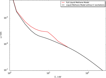
Figure 5. Plot of the resistivity curve for liquid methane at 422 kg m−3 as calculated by the full model, and the model without electron impact excitation of carbon ions/atoms.
Download figure:
Standard image High-resolution imageFigure 5 clearly shows that C excitations strongly affect the resistivity in the 3–20 eV range in liquid methane as well as polyethylene and vitreous carbon. In figure 6 we compare the three resistivity curves generated by the full models (i.e. including C excitations) for vitreous carbon, polyethylene and liquid methane.

Figure 6. Plots of the resistivity curves for vitreous carbon, polyethylene at 1000 kg m−3, and liquid methane at 422 kg m−3 as calculated by the full model for comparison.
Download figure:
Standard image High-resolution image
This shows that the resistivity of liquid methane follows that of polyethylene very closely, but the resistivity of both behaves substantially different from that of vitreous carbon. The reason for this being the difference in the temperature dependence of the ionization state of carbon in the hydrogen bearing versus the pure carbon materials.
4. Conclusions
In this paper we have presented a resistivity model for non-crystalline carbon and hydrocarbons in the 1–100 eV range. Importantly we have included electron-impact excitation of C atoms and ions in this model and have shown that this has a strong effect on the resistivity. In the 3–20 eV region accounting for electron-impact excitations of C leads to an increase in the calculated resistivity by a factor of 2–3. This conclusion is supported by a comparison between the model prediction and DF-QMD calculations of the resistiviy of vitreous carbon.
Such a difference in the resistivity is far from negligible when it comes to interpreting ultra-intense laser-solid experiments, and this may well have implications for some of the proposed applications of laser-solid interactions. The possibility of electron-impact excitations being so prominent was not discussed in previous studies [29]. The widely used Lee–More model [24] did not include electron-impact excitation, only accounting for electron–ion and electron–neutral scattering. In an improved version of the Lee–More model (Lee–More-Desjarlais), Desjarlais [25] also included electron–electron scattering. However such inelastic processes were still not included. The results that we present here indicate that excitation processes are important for solid density carbon and hydrocarbon in the 3–20 eV range. Studies of the transport of laser-generated fast electrons in both carbon and silicon [18, 41] indicate that this 'low temperature' or 'WDM' regime is highly important to understanding the transport of fast electrons, and we therefore believe that the results of this study will be of benefit to this research area. Furthermore these results suggest that the resistivity of many other non-crystalline materials in this temperature range will be affected by excitation processes. Further work is required to produce similar resistivity models and to understand the implications.
Acknowledgments
This work was supported by the European Research Council's STRUCMAGFAST grant (ERC-StG-2012). APLR and HS are grateful for the use of computing resources provided by STFC's Scientific Computing Department.