


Abstract
We investigate an artificial molecular dimer made of two dipole coupled cyanine dye monomers in which a strong coherent coupling between electronic and vibrational degrees of freedom arises. Clear signatures of this coupling are reflected in an oscillatory time evolution of the off-diagonal vibronic cross peaks in the two-dimensional optical photon echo spectrum. We find a strong coherence component damped by fast electronic dephasing ( fs) accompanied by a much weaker component which decays on the longer time scales (ps) associated to vibrational dephasing. We find that vibronic coupling does not cause longer dephasing times of the dominant photo echo component but additional weak but long-lived components emerge.
Export citation and abstract BibTeX RIS
1. Introduction
Over the last several years, multidimensional ultrafast optical spectroscopy has been developed into a very successful probing tool [1–4] aiming to reveal quantum coherent dynamics of excitonically coupled electronic states. The femtosecond time scale of the excitonic dynamics in photoactive molecular compounds and, especially, in natural photosynthetic units such as the antennae complexes and the reaction centers has become accessible (see e.g. [3, 5–8]).
While some two-dimensional (2D) spectra at low temperature clearly display excitonic features in the form of well-resolved spectroscopic cross peaks [3, 6], at ambient temperature they are often fairly unstructured, and recovering of useful information about exciton states and their couplings is not possible. However, it has been reported that the measured sequences of 2D spectra taken at different 'waiting' time delays T contain periodic oscillations in their amplitudes. Recent examples include the Fenna–Matthews–Olson (FMO) complex [9, 10], photoactive marine cryptophyte algae [5], the bacterial reaction center and the light-harvesting complex LH2 of Rhodobacter sphaeroides [11, 12], the light-harvesting complex LHCII of the Photosystem II [6], and chlorosomes from the green sulfur bacterium Chlorobaculum tepidum [13]. Strong long-lived oscillatory components have been recently observed in the 2D photon echo spectra of artificial units at room temperature in J-aggregates [14]. These oscillations were initially attributed to the strong quantum coherent coupling between the excitonic states formed by interacting electronic states of the molecules [5, 10]. However, in addition to the purely electronic couplings [15], signatures of the vibrational degrees of freedom of the pigment-protein host [16] can also be accessed on the same spectroscopic footing. Any coherent coupling in general shows up in a sequence of 2D spectra in form of a coherent oscillatory time evolution of the amplitude of off-diagonal cross peaks. Long-lived purely electronic coherences are unexpected and have been proposed to affect the mechanism, the quantum yield, and the time scale of light harvesting [17–21]. However, long-lived vibrational coherences are common and are not expected to strongly affect the light harvesting. Identifying the nature of this coherence, specifically the details of the involvement of vibrational effects into the excitonic dynamcis, has thus become a hotly debated issue [19, 22–36].The decoherence rate reflects the magnitude of frequency fluctuations which arise from the coupling to the surroundings. Vibrational transitions have small fluctuations since the solvent interactions are not very sensitive to the vibrational state. However, electronic transitions show much stronger fluctuations, hence the faster decoherence (see chapter 5 and 6 in [37]).
When the coherent coupling of the electronic and vibrational degrees of freedom exceeds the linewidth of the involved states, the individual degrees of freedom lose their meaning and, typically, the system is called vibronic. Both the electronic and the vibrational branches are coupled to different environments (e.g. bulk solvent polarization fluctuations or vibrational fluctuations of the protein structure) with different coupling strengths. However, in the presence of a strong coherent vibronic coupling, the nontrivial question arises: how do the different environmental sources affect the overall quantum coherent vibronic features [38, 39]? So, for instance, could a weak vibrational decoherence suppress strong electronic coherence via the mutual coupling? Naively, one expects that the coupled vibronic states are now all affected by the electronic transition fluctuations and, thus, all decay fast.
Natural molecular complexes are rather large and involve many neighboring excitonic states, broad spectral line shapes, and a complicated spectrum of vibrational modes. In turn, the ensuing strong spectral overlap of the excitonic and vibrational degrees of freedom renders it challenging to identify strongly overlapping cross peaks in the 2D-spectra. Thus, to pinpoint the nature of the coherence, an artificial model dimer which is much less complex in the electronic and vibrational structure and can be chemically synthesized in a controlled way, is highly desirable. Such a 'sandwich'-like homo-dimer of two identical indocarbocyanine molecules bound by two butyl chains (compound A-5 of [40]) is available together with the measured data of linear spectroscopy, and forms the basis of our work. The 2D spectroscopy measurements of this compound, dissolved in methanol, were recently reported [41, 42]. Due to the strong excitonic coupling, the absorption spectrum of the dimer shows strong and well-resolved peaks, which are accompanied by well-resolved cross peaks in the 2D spectra. Moreover, the fixed distance and angle between the monomers significantly suppress conformational variations throughout the sample. We note that this dimer forms an H-aggregate, where the lower (in energy) excitonic state has a much lower transition strength. For the given geometry with the angle between the transition dipole moments of the monomers of 15°, it is approximately  of the main transition strength. The strongest peaks observed in the dimer absorption spectrum contain also significant contributions from the vibrational states, strongly mixed with the pure electronic transitions
  [43, 44].
In this work, we rigorously establish a vibronic exciton model, i.e. the need for a strong electron–vibration coupling in order to reproduce the experimentally measured absorption spectra of both the monomer and dimer. We-find well-separated peaks also in the calculated 2D photon echo spectra. These spectra agree well with experiment [41, 42]. On the basis of this accurate modeling of the real molecular complex, we show that the strong vibronic cross peaks, which occur in the 2D spectra, evolve in a quantum coherent manner over the electronic decoherence time (about of ∼50 fs). Their oscillation periods correspond to the vibronic splittings. Moreover, the theoretical model allows us to vary the angle between transition dipole moments of the two monomers 'in theory' in a controlled way. This modifies the vibrational contributions to the exciton states and proves that the overall decoherence is dominated by the electronic dephasing. Likewise, it is essentially independent of the vibrational dephasing channel. These findings fully express the naive expectation that all vibronic states are subject to electronic dephasing and, thus, correspoding 2D signals must decay fast. Surprisingly, there is additionally a small slowly decaying oscillatory component which we observe by extending our simulations to delay times up to 400 fs. Its oscillation frequency exactly corresponds to the frequency of the vibrational transitions and their decay is caused by the weak vibrational decoherence and typically last up to several picoseconds for the C-C stretching mode. The associated frequency of  cm−1 is determined by a weak delocalization with the electronic states. Thus, the overall kinetics of the spectral cross peaks has two clearly separated and distinguishable contributions: (i) dominant strongly damped (short-lived) components, and (ii) underdamped long-lasting oscillations due to vibrational decoherence.
2. Model
2.1. Monomer
To construct the model, we start with the monomer and set up a Hamiltonian which includes vibrational states. By an accurate fit to the experimental absorption spectrum, we determine its parameters. We consider an electronic transition between the electronic ground S0 ( ) and first excited state S1 (
 ), separated by the energy gap E. The electronic states are coupled to the excitations of a single vibrational harmonic mode with the frequency Ω and with the bosonic creation and annihilation operators
  and b, respectively. We denote the exciton–phonon coupling constant by λ. The monomer Hamiltonian thus reads (
 )
)

with  and
and  . We further couple the monomer Hamiltonian to a fluctuating Gaussian quantum mechanical environment described by the Hamiltonian
  [45]. The bilinear coupling is given by
  . The excited electronic state is coupled to the quantum statistical fluctuations via
  , while the vibrational motion is coupled to a different harmonic bath via
  . Both baths have the same Ohmic spectral density, i.e.
  . We assume a large cut-off frequency
  taken to be equal for both branches but different coupling strengths
  . We calculate first the absorption spectrum [46]

For the monomer  is the respective transition dipole moment operator. The quantum dynamics was calculated by means of the time-nonlocal master equation [47] for the system's reduced density operator
  after tracing out the bath degrees of freedom (for details of the calculation, see the supplementary information (SI)). The subscript g in equation (2) indicates a tracing with respect to the initial state given by the equilibrium density operator (kB = 1)
  with
with  where the vibrational mode is in thermal equilibrium at temperature
  K. The electronic and the vibrational bath are held at the same temperature. Inhomogeneous broadening was included by convoluting the calculated homogeneous absorption spectrum of equation (2) with the Gaussian-shaped inhomogeneous broadening function. Note that we include inhomogenous broadening for the 2D spectra and the absorption and 2D spectra for the dimer discussed later also by convoluting the final spectra with the Gaussian. Furthermore, the obtained spectra for the monomer, as well as the 2D spectra and the absorption and 2D spectra for the dimer discussed later, are averaged over random orientations. From the fitting of the calculated absorption spectrum to the experimental one, we obtain the complete set of parameters for our model: E = 18850 cm−1,
  cm−1,
cm−1,  cm−1,
cm−1,  ,
,  ,
,  cm−1, and the FWHM of the inhomogeneous broadening of 300 cm−1 which is typical for the dissolved organic dyes at room temperature. Our model reproduces the monomer experimental absorption spectrum very well as shown in figure 1(a), together with the calculated stick spectrum. For achieving convergent results, we have included
  vibrational eigenstates. To estimate the vibrational dephasing rate, we first set
  and kept the off-diagonal elements of the vibrational coupling in the exciton representation. Then, using an estimated vibrational lifetime of 1 ps, we have adjusted the vibrational dephasing rate to
  . The stick spectrum in figure 1(a) clearly shows that the main peak is purely electronic, while the three well-resolved side peaks have a vibrational origin (see the SI for details).

Figure 1. Measured (symbols) and calculated (lines) absorption spectra of the monomer (a) and dimer (b). In addition, the stick spectra are shown. The electronic and vibrational contributions to the eigenstates are indicated by the different colors. The main electronic transition in the monomer spectrum (the 'zero–zero' transition), as well as the vibrational progressions, are clearly resolved. In the dimer spectrum (b), a clear electron–vibrational coherent coupling is present. The green line in (b) indicates the power spectrum of the excitation pulse of the laser used in the simulations.
Download figure:
Standard image High-resolution image2.2. Dimer
Having obtained the monomer model parameters, we next turn to the dimer. It consists of two identical indocarbocyanine monomers, covalently bounded by two butyl chains (the homodimer) with an in-plane angle of  . To extend our model for the dimer, we use the Hamiltonian

Note that each monomer has its own baths. Here, U is the electronic dipole coupling which can be calculated in the point–dipole approximation using a structural information for the dimer skeleton, obtained using the HyperChem v.7 package (for details, see the SI). For this geometry, the calculated value of U is  cm−1. The dimer Hamiltonian includes two vibrational modes each belonging to one monomer in the same way as the molecular Hamiltonian. Hence,
  and
and  for the ground and excited states, respectively. The total transition dipole moment is
  with
with  and
and  with angle α between the dipole moments and
  the unit vectors in the coordinate system of the dimer. The dimer absorption spectrum was also calculated using equation (2). The excellent fit to the experimental spectrum is depicted in figure 1(b). We used the parameters E = 18700
 cm−1, and
  cm−1. The slight modification of the monomer parameters (which have been used as an initial guess in the fitting procedure) is reasonable and could be attributed to the presence of the butyl chains perturbing the wave functions of the monomers. We have used the same values for the damping parameters as for the monomer. The stick spectrum in figure 1(b) reveals a strong electron–vibrational coherent coupling6
. Different states have quite different vibrational/electronic contributions in the stick components (for details of the calculations, see the SI). For example, the main peak labeled as A shows almost equal contributions from electronic and vibrational states. For peak C, the electronic contribution is dominant, whereas the vibrational contribution clearly dominates in the peak B. From the electronic and vibrational contributions to the eigenstates, depicted on the stick spectrum in figure 1(b) using different colors (see figure caption), one already could expect that the dephasing of the associated transitions, and consequently the damping of coherent oscillations in the 2D spectra, should be rather different since the dephasing of pure electronic transitions is in general much stronger than the vibrational dephasing. However, as we will demonstrate below, this is not the case.
cm−1. The slight modification of the monomer parameters (which have been used as an initial guess in the fitting procedure) is reasonable and could be attributed to the presence of the butyl chains perturbing the wave functions of the monomers. We have used the same values for the damping parameters as for the monomer. The stick spectrum in figure 1(b) reveals a strong electron–vibrational coherent coupling6
. Different states have quite different vibrational/electronic contributions in the stick components (for details of the calculations, see the SI). For example, the main peak labeled as A shows almost equal contributions from electronic and vibrational states. For peak C, the electronic contribution is dominant, whereas the vibrational contribution clearly dominates in the peak B. From the electronic and vibrational contributions to the eigenstates, depicted on the stick spectrum in figure 1(b) using different colors (see figure caption), one already could expect that the dephasing of the associated transitions, and consequently the damping of coherent oscillations in the 2D spectra, should be rather different since the dephasing of pure electronic transitions is in general much stronger than the vibrational dephasing. However, as we will demonstrate below, this is not the case.
3. Results: 2D spectra
3.1. Short waiting times
We next address the coherent time evolution of the coupling of electronic and vibrational degrees of freedom in the artificial dimer. To that end, we consider the 2D photon echo spectrum [1, 2, 4] which can be calculated using the phase matching approach of [48] in combination with the time-convolutionless quantum master equation [47]. The doubly excited states (the excited-state absorption) with an exciton at each monomer were properly accounted for in the model calculation but doubly excited states within the monomers were neglected. To match the experimental conditions, the carrier frequency of the laser pulse is set to 18520 cm−1 and its duration to a FWHM of 7 fs. The resulting 2D photon echo spectra at different waiting times T are shown in figure 2. We see clearly separated diagonal peaks which correspond to the peaks  and C in the linear absorption spectrum shown in figure 1(b). We note that the peak A represents a strong electron–vibrationally superposed state. Also, well-separated cross peaks (labeled by D to I) appear. Peaks D and G are the most intense and correspond to the interference between the diagonal peaks A and B.
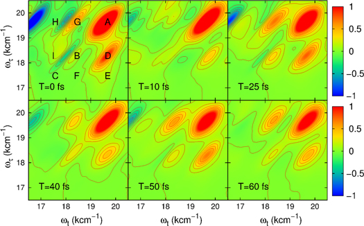
Figure 2. Real part of 2D photon echo spectra of the dimer at different waiting times (as indicated) calculated with the model parameters obtained from the fit of the dimer linear absorption spectrum. The diagonal as well as the cross peaks are labeled by capital letters in the frame T = 0 fs.
Download figure:
Standard image High-resolution imageThe strong vibronic coherent coupling is further illustrated in the sequence of 2D spectra for increasing waiting times with step of 10 fs, shown in figure 2. We can clearly identify the oscillatory behavior of the amplitudes of the cross peaks by eye. The calculations reproduce well the main features of the measured 2D spectra [41, 42]. The slight underestimation of the excited state absorption is likely due to neglecting the higher excited states of the monomer.
To study the effect of the environment on the coherent coupling in more detail, we monitor the time evolution of the amplitude of the cross peaks as labeled in figure 2 for increasing waiting times. They can readily be extracted from the series of the 2D spectra (the calculations were performed with the waiting time step of 5 fs). The results are shown in figure 3 as symbols to which we fit a cosine function damped by a single exponential decay (solid lines, the details of the fitting procedure are given in the SI). This yields the oscillation periods and decay times which are summarized in table 1 (first row). We find that the coherent oscillations appear with a period of around 25 fs and with decay times of 40–50 fs. The latter are typical electronic dephasing times of organic dyes. The oscillation frequencies match the energy splittings between the main transitions A, B, and C in the dimer absorption spectrum (figure 1(b) given by the stick components. Likewise, the coherence time (i.e. the decay time of the oscillations  in table 1) is clearly dominated by the electronic dephasing for all cross peaks. More importantly, these coherences are independent of the participation ratio between the electronic and vibrational contributions. This can be additionally verified by increasing the vibrational dephasing rate by one order of magnitude. The system then goes from the regime of weak damping with
  to the regime of intermediate damping with
  . We find a proportional decrease of the vibrational coherence time from 2 ps to
  fs. The extracted oscillations for both cases are also plotted in figure 3. For this intermediate damping, we find similar coherent oscillations decaying within a similar time window. The resulting fit parameters to the exponentially decaying cosine function are given in table 1 (second row). Up to minor quantitative (on the order of 1) modifications, no significant impact of the increased vibrational damping is observed. This shows that the amplitude of the oscillating cross peaks is damped by the strong fluctuations acting on the electronic degree of freedom, i.e. electronic dephasing and, importantly, the weak vibration–bath coupling cannot reduce its damping.
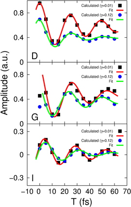
Figure 3. Amplitude of the spectral cross peaks  and I versus the waiting time T. The symbols mark the cross peak maxima extracted from the real parts of the 2D spectra, while the solid lines represent a fit to an exponentially decaying oscillatory function. The oscillatory behavior of the cross peaks is shown for both the weakly (
 ) and the intermediately (
 ) damped vibrational modes (see text for details).
Download figure:
Standard image High-resolution imageTable 1.
Oscillation periods TX and decay times  of the cross peak maxima for the peaks
  and I for a weakly damped vibrational mode with
  (case I) and an intermediately damped vibrational mode with
  (case II).
| D | G | I | ||||
|---|---|---|---|---|---|---|
| Case | TD/fs | τD/fs | TG/fs | τG/fs | TI/fs | τI/fs |
| I | 24.6 ± 0.64 | 39 ± 8 | 28 ± 2.7 | 26 ± 12 | 24.8 ± 0.8 | 38 ± 13 |
| II | 26 ± 1.6 | 19 ± 4 | 26.7 ± 1 | 30.5 ± 12 | 26.8 ± 1.3 | 24 ± 7.6 |
Further proof can be obtained by changing the angle α between transition dipole moments of the monomers. This is readily possible in our accurate theoretical model while it could be a great challenge in the experiment. Tuning of α modifies the exciton coupling between molecules, changes the relative intensities of the excitonic transitions, and induces a redistribution of the electronic contributions relative to the vibrational ones. For example, for  , the ratio of the peak amplitudes of A and C in the absorption spectrum reaches
  versus
  for
for  . Thus, tweaking of α permits an easy control of the exciton transitions and of the contributions to both the electronic and vibrational sector. Some examples of calculated absorption and stick spectra with corresponding electronic and vibrational contributions for different α are given in the SI.
We have calculated 2D spectra for various angles and waiting times increasing in steps of 5 fs. From there, the time dependence of the cross peaks was extracted and fitted to a single exponentially decaying cosine function as before. The results of this fitting for the cross peaks D and G are collected in figure 12 in the SI. We find that despite small quantitative changes, the decay times are essentially independent from the angle α between the monomer transition dipole moments. This supports the previous conclusion that the quantum coherence of excitonic transitions is clearly dominated by the electronic dephasing. It is well established that in some excitonically coupled systems the coherent oscillations in measured 2D spectra live sometimes significantly longer than primitively estimated from the magnitude of electronic dephasing. This is true even at room temperature (see e.g. [5, 10, 14]). Nevertheless, their magnitudes are rather weak. In the recent experimental study [11] of the oxidized reaction center from Rhodobacter sphaeroides, which can be considered as a good 'natural' dimer model, the authors found in the 2D spectra weak oscillations lasting up to 1 ps at room temperature. Therefore, the origin and the physical mechanism of such long-lasting oscillations needs to be established.
3.2. Long waiting times
In our search for weak but long-lived oscilationary components, we have extended the waiting time window in our simulations to 400 fs and have found that, alongside with the short-lived oscillations in the cross peaks analyzed above (figure 3), there are much weaker long-lived oscillations. A typical example of these oscillations for our model dimer with  and
and  for the cross peak D is shown in figure 4. In this case, we fit this dynamics with two decaying cosine functions (see the SI for details) and find two similar yet distinguishable periods. The period of the strongly damped oscillation corresponds to the splitting between the interfering diagonal peaks A and B in the time domain, whereas the period of the long-lived oscillation precisely corresponds to the value of the vibrational frequency of
  cm−1. For this particular cross peak D, the ratio between their amplitudes is
  and is different for the other cross peaks. Notably different is the ratio for the imaginary part of the oscillations in the selected cross peak (see also figure 4). The long-lived component is stronger by about one order of magnitude. Since the overall amplitude of the real part dominates, the absolute 2D spectrum only shows a weak component of long-lived oscillations. Thus, it might be experimentally advantageous to study 2D phase-resolved spectra.
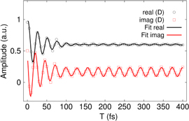
Figure 4. Oscillations in cross peaks D in a large waiting time window (symbols) and results of two-component fit (see in text) revealing oscillatory frequencies 1235 ± 30 and 1350 ± 28 cm−1 corresponding to the vibrational frequency Ω and to split between peaks A and B in the absorption spectrum of dimer, respectively.
Download figure:
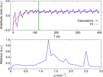
Standard image High-resolution imageWe observe a similar mixing of a strongly damped oscillation with a period corresponding to the splitting between peaks A and B and the long-lived vibrational frequency Ω (figure 5) for the position in the 2D spectra with  cm−1 and
  cm−1, labeled in [41] as peak X. The calculated kinetics is in good agreement with the experimental observation (see figure 4(d) in [41]). The measurement along with its theoretical description in [41] was performed in a much smaller waiting time window (120 fs) than we used in our simulations (400 fs). Figure 4 clearly resolves that at waiting times around 100 fs both contribution are of the same order of magnitude. Data up to this point does not justify a fit with two separate components and a fit with only a single component results only in a slightly longer dephasing time (as observed in [41]) than in our analysis for the strong component obtained. Moreover, the polaron-like model used in [41] in which the vibrational mode has been integrated out generates an additional mixing of the contributions which renders the separation more difficult. Thus, our extended simulation (fully in line with experiments up to waiting times of ∼100 fs) reveals the long-lived weak component as a theoretical prediction to be tested in an experiment.
Figure 5. Kinetics of 2D spectra (top) for the peak position of  cm−1 and
  cm−1. The vertical line marks the time delay window used in the experiment in [41]. The Fourier transform of residuals (bottom) after a 3-exponential fit of kinetics reveals fast-decaying and long-lasting oscillations with the frequencies of
  cm−1, a vibrational frequency
  cm−1, and a high-frequency component
  cm−1 originating in the excited-state absorption. While the 1400 cm−1 component has a rather broad spectral width, the accompanied vibrational component is very narrow.
Download figure:
Standard image High-resolution image
The nature of this long-lived oscillation becomes clear if we investigate more precisely the absorption stick spectrum as shown in the inset of figure 1(b). The small satellite in the vicinity of the stick A has in essence a pure vibrational origin and the contribution of electronic transitions is very small. In turn, its decoherence is weak and the split between the stick component B and this satellite is precisely given by Ω. Therefore, their interference generates a long-lived oscillation with the frequency being equal to the vibrational frequency Ω and with a weak amplitude which is dictated by the small magnitude of that satellite.
To confirm this result, we have examined several additional parameter combinations. We have doubled the vibrational frequency and have kept all other model parameters unchanged. Similarly, we have decreased the excitonic coupling strength to U = 250 cm−1 and kept the vibrational frequency at the previous value of  cm−1. In all cases, we have found long-lasting oscillations with small amplitudes in the kinetics of the cross peaks in addition to the quickly decaying short-time oscillations. All results are consistent with those shown in figures 3 and 4. Importantly, the frequencies of the low-amplitude oscillations coincide with the vibrational frequency used. Whereas in the experimentally studied dimer both the energy difference between peak A and B and the vibrational frequency are very similar, in these theoretically designed dimers these energies differ strongly and, thus, this assignment is unambiguous.
3.3. Perturbative estimates
This observation of an accurate coincidence of the frequencies of the long-lived oscillations and vibrational states can be understood using lowest-order perturbation theory. For the two equal monomers making a dimer, standard perturbation theory for degenerate states yields a contribution in first order in U, while the electron–phonon coupling appears only in second order in g. We find for the dimer energies of the state  the expressions
  ,
,  and
and  . Since these expressions only include the lowest order contributions, they can provide only the location of those peaks whose electronic or vibrational contribution is sizable. Inserting the values obtained from a fit to the linear absorption spectrum from above, we find the peaks at energies given by
  cm−1,
cm−1, 
 cm−1 and
  cm−1. Also, the peaks at higher energies
  are present, although they are significantly smaller in amplitude. They follow as
  cm−1,
cm−1,  cm−1,
cm−1,  cm−1 and
  cm−1. Fair enough, the accuracy of this lowest-order estimate is limited. Moreover, additional tiny peaks in the absorption spectrum are not covered by the lowest-order estimates of the energies and higher orders are required.
4. Conclusion
In summary, we have provided an accurate microscopic study of the coherence dynamics in a model dimer formed by two identical indocarbocyanine dye molecules in the presence of a diabatic quantum coherent vibrational mode. We have established a quantitative model based on two excitonically-coupled monomers each coupled to a single vibrational mode. The model parameters are determined by a quantitative fit to the absorption spectra of the monomer and the dimer. We find a strong coherent electronic–vibrational coupling which is also reflected in the coherent time evolution of the cross peaks. We, therein, observe a dominant contribution which is subject to electronic dephasing and thus decays on a time scale of  fs. No substantial increase of this dephasing time is observed for any parameter variation we studied. Thus, substantial enhancement of the coherence time due to vibronic coupling is not observed. Additionally, however, we find a weak component with decay times of the order of picoseconds as known for vibrational damping. The according oscillation frequency is identical to the frequency of the vibrational mode even when artificially modifying the vibrational frequency, the excitonic coupling or the angle between the dipoles. Thus, this long-lived part results from a component dominated by the vibrational degree of freedom. These results prevail qualitatively also when studying heterodimer with energy differences of up to
  cm−1 of the monomers (data not shown).
Our findings are fully in line with experimental 2D spectra [41] of our studied dimer system up to the experimentally studied waiting times of ∼120 fs and predict weak long-lived oscilatory cross peaks for longer times. Additionally, the results propose a picture for the oscillations observed. The observed oscillations in the cross peak amplitudes in the 2D photon echo spectra are generated by a superposition of several components of the wave functions with different origins. They can be conditionally separated into two groups. (i) The short-lived and large-amplitude oscillations which are rapidly damped due to a strong electronic dephasing. The associated frequencies are determined by the vibronic splittings. In addition, (ii) there exist long-lasting, but small-amplitude oscillations whose life times and frequencies are determined by the inherent properties of the molecular vibrational states. Our results suggest a similar picture for the oscillatory behaviour observed in photosynthetic complexes.
Finally, we note that the polarization of light is another control knob that may be used to distinguish between electronic and vibrational relaxation channels. Four polarizations can be independently varied in a four-wave mixing experiment. These could be optimized to reveal the desired features. This will be an interesting possibility to explore in the future.
Acknowledgments
We acknowledge financial support by the Joachim-Herz-Stiftung, Hamburg, within the PIER Fellowship program and by the excellence cluster 'The Hamburg Center for Ultrafast Imaging— Structure, Dynamics and Control of Matter at the Atomic Scale' of the Deutsche Forschungsgemeinschaft. S M gratefully acknowledges the support of the National Science Foundation through grant no. CHE-1361516, and the Chemical Sciences, Geosciences and Biosciences Division, Office of Basic Energy Sciences, Office of Science, US Department of Energy.
Footnotes
- 6
We note a significant difference between the stick-spectrum obtained from our model which is based on a rigorous molecular Hamiltonian, and the calculated one in [41].