A gauge invariant theory for time dependent heat current

The Onsager relation [1] is one of the most important relations in quantum transport, which is related to the equilibrium fluctuation dissipation theorem. For DC charge transport, the linear conductance in the presence of a magnetic field satisfies ${{G}_{\alpha \beta }}(B)={{G}_{\beta \alpha }}(-B)$ as a result of microscopic reversibility. In the nonlinear DC charge transport, the departure of the Onsager relation was investigated [2]. In the nonlinear regime, the self-consistent Coulomb potential has to be included in order to preserve the gauge invariance [3]. As interpreted in [2], the Coulomb potential is not an even function of the magnetic field, which is responsible for the departure of the Onsager relation. In the linear regime of AC charge transport, the self-consistent Coulomb potential is still needed to satisfy the current conserving and gauge-invariant condition [3]. In this case the Onsager relation is shown to hold, even though the Coulomb potential is not an even function of the magnetic field [4]. In addition to the charge, the flow of electrons also carries energy that produces the heat current. In the DC case, the Onsager relation holds in the linear regime for the heat current and is violated in the nonlinear regime due to the presence of the self-consistent Coulomb interaction. However, whether the Onsager relation is valid for AC heat transport remains to be answered, since a self-consistent theory for AC heat current has not been formulated. It would be interesting to address this issue.

As electrons traverse the scattering region, both electric current and heat current are generated. The investigation of heat current has attracted a lot of attention. The multi-channel Landauer formula for thermoelectric transport was derived [5] in 1986 and later cast into a scattering matrix formalism [6]. This formalism allows us to study both electric and heat transport as well as thermoelectric transport where a temperature gradient is present. Recently the efficiency of nanoscale heat engines has been the focus of intense study where heat current is driven by both bias voltage and temperature difference [7, 8]. Recently, the heat current has been studied in the context of full counting statistics, where a generating function for the heat current was calculated [9]. This enables one to study the efficiency fluctuation of heat engines at nanoscale, which may characterize the performance of nano heat engines more accurately [9].

So far most of the investigations focus on DC heat transport; less attention has been paid to AC heat transport [10]. Using the time-dependent scattering matrix, Moskalets and Buttiker [11] discussed the heat flow and the quantum statistical noise properties of an adiabatic quantum pump at finite temperature. Wang and Wang have studied the heat current in a parametric quantum pump and derived a general formula for pumped heat current at finite frequency and pumping amplitude [12]. Comparing the heat current generated by the adiabatic quantum pump with the Joule heat dissipated during the pumping process, Avron et al found a general lower bound for the heat current [13]. This concept of optimal pump has been generalized to the parametric quantum pump connected by a superconductor lead [14]. The heat current through a carbon nanotube-based quantum pump has been explored by calculating the heat current order by order in pumping amplitude at finite frequencies, where the photon-assisted process has been found [15]. Recently, dynamic thermoelectric and heat transport properties in mesocopic capacitors have been studied using the scattering matrix theory [16]. The Coulomb interaction was considered similar to the approach of reference [17], where a constant Coulomb potential was assumed. It was found that by tuning the gate voltage, the thermocurrent can lead or lag the applied temperature. In addition, the relaxation resistance of the heat current due to the temperature gradient is found to be a universal value–half of the thermal resistance quanta. Dynamic energy current has also been investigated within the scattering matrix theory, and new energy reactance was identified [18]. Furthermore, heat current noise was investigated using the scattering matrix theory [19, 20]. We note that in all these works, except reference [16], the self-consistent Coulomb interaction has not been considered.

First principles calculations using density functional theory (DFT) within the framework of a non-equilibrium Green's function method (NEGF) have been carried out to a make quantitative prediction of DC charge transport properties for nano-devices [21–23]. The formalism has been extended to calculate the AC charge current [24]. How to extend the NEGF-DFT formalism to treat AC heat current carried by electrons from first principles is still an open question. The aim of this paper is to develop a theoretical formalism for heat current under AC bias in the absence of electron–phonon interaction, using an NEGF theory that will pave the way for first-principles heat current investigation.

It is known that the self-consistent Coulomb interaction should be included in order to satisfy two basic requirements for the AC charge transport: gauge invariance and current conservation [3, 17]. In electronic heat transport, the gauge-invariant condition must be satisfied, while the heat current may not be conserved due to dissipation. We show in this paper that the self-consistent Coulomb interaction must be included in order to satisfy the gauge-invariant condition. Since the self-consistent Coulomb potential depends on time explicitly, there is no closed-form solution for heat current at finite frequency and finite bias. In this paper we use the perturbation approach and expand frequency-dependent heat current in terms of external bias so that frequency-dependent Coulomb potential can be considered. As an example, we obtain a general expression for the frequency-dependent electrothermal admittance with the Coulomb interaction included. Higher-order nonlinear electrothermal admittance can be calculated in a similar fashion. We also examine the validity of the Onsager relation for the electrothermal admittance and find that it is valid only for a special case for a quantum dot with a single energy level when a quasi-neutrality condition is assumed. Finally, we have applied our theory to a nanocapacitor. We note that an important physical ingredient in the case of a nanocapacitor is the electron–electron interaction [3]. For macroscopic metal plates this interaction is largely screened, but for nanoplates where the DOS is low, the screening length can be long enough to play an important role, leading to a quantum correction to capacitance. The analytic expression for heat current is obtained using the discrete potential model. We find that the heat current is related to the electrochemical capacitance, up to the first order in frequency.

This paper is organized as follows. In section 2, for a multi-terminal mesoscopic system we present a gauge-invariant AC theory for heat current, taking into account the self-consistent Coulomb interaction. DC theory is recovered as the frequency of bias voltage goes to zero. The gauge-invariant condition and the Onsager relation are examined in the DC limit. In section 3, a general expression for the frequency-dependent heat current is derived based on the non-equilibrium Green's function, including the self-consistent Coulomb potential in the linear regime. The departure of the Onsager relation for the electrothermal admittance is discussed. In section 4, the heat current of nanocapacitors is calculated. To obtain an analytic solution, a discrete potential model is used. Finally, a brief summary is given in section 5.

We consider a multi-terminal system consisting of a central scattering region connected by N leads labeled by α to the outside reservoirs, where AC bias $q{{v}_{\alpha }}{\rm cos} \omega t$ is applied at the αth lead. The Hamiltonian of this system can be written as ($\hbar =1$ ):

$$\begin{eqnarray}&&\hat{H}(t)=\mathop{\sum }\limits_{\alpha }{{H}_{\alpha }}(t)+{{H}_{dot}}(t)+{{H}_{T}}(t)\end{eqnarray} \tag{ 1 }$$

and,

$$\begin{eqnarray}&&{{H}_{\alpha }}(t)=\mathop{\sum }\limits_{k}{{\epsilon }_{k\alpha }}(t)a_{k\alpha }^{\dagger }{{a}_{k\alpha }}\end{eqnarray} \tag{ 2 }$$

$$\begin{eqnarray}&&{{H}_{dot}}(t)=\mathop{\sum }\limits_{n}{{\epsilon }_{n}}(t)d_{n}^{\dagger }{{d}_{n}}+\mathop{\sum }\limits_{nm}{{V}_{nm}}d_{n}^{\dagger }{{d}_{n}}d_{m}^{\dagger }{{d}_{m}}\end{eqnarray} \tag{ 3 }$$

$$\begin{eqnarray}&&{{H}_{T}}=\mathop{\sum }\limits_{k,n,\alpha }[{{t}_{k\alpha n}}a_{k\alpha }^{\dagger }{{d}_{n}}+h.c.]\end{eqnarray} \tag{ 4 }$$

where ${{H}_{\alpha }}$ describes the non-interacting electrons in the lead α with ${{\epsilon }_{k\alpha }}(t)=\epsilon _{k\alpha }^{0}+q{{v}_{\alpha }}{\rm cos} \omega t,$ and $a_{k\alpha }^{\dagger }$ $({{a}_{k\alpha }})$ is the creation (annihilation) operator in the corresponding lead α with the electronic state labeled by k. The second-term H_dot stands for the quantum dot, and $d_{n}^{\dagger }$ $({{d}_{n}})$ creates (annihilates) an electron in the quantum dot. The electron–electron interaction is included in H_dot. The third-term H_T represents the coupling between the quantum dot and the lead with the coupling constant ${{t}_{k\alpha n}}.$ We will work at low temperatures so that the influence of electron–phonon interaction is less important and can be neglected.

2.1. Coulomb interaction

The electron–electron interaction is taken into account in the second term of equation (3) in H_dot, where V_nm is the matrix element of the Coulomb potential and is given by $V(x,x^{\prime} )=1/|{\bf x}-{{{\bf x}}^{\prime }}|$ in real space. In the Hartree approximation, equation (3) can be simplified as [4]

$$\begin{eqnarray*}&&{{H}_{dot}}=\mathop{\sum }\limits_{n}({{\epsilon }_{n}}+{{U}_{n}})d_{n}^{\dagger }{{d}_{n}}\end{eqnarray*}$$

where

$$\begin{eqnarray}&&{{U}_{n}}=\mathop{\sum }\limits_{m}{{V}_{nm}}\langle d_{m}^{\dagger }{{d}_{m}}\rangle .\end{eqnarray} \tag{ 5 }$$

Recalling the definition of the lesser Green's function, $G_{nn}^{\lt }=i\langle d_{n}^{\dagger }{{d}_{n}}\rangle$, we can rewrite equation (5) in real space as

$$\begin{eqnarray*}&&U(x)=-i\int {\rm d}x^{\prime} V(x,x^{\prime} ){{G}^{\lt }}(x^{\prime} ,x^{\prime} )\end{eqnarray*}$$

from which we obtain the Poisson equation

$$\begin{eqnarray}&&{{\nabla }^{2}}U(x,t)=-4\pi \rho (x,t)=-4\pi iq{{[{{G}^{\lt }}(t,t,U)]}_{xx}}.\end{eqnarray} \tag{ 6 }$$

Making a double-time Fourier transform with respect to time on equation (6), we find

$$\begin{eqnarray}&&{{\nabla }^{2}}U(x,\Omega )=-4\pi {\rm i}q\int ({\rm d}E/2\pi ){{[{{G}^{\lt }}(E+\Omega ,E,U)]}_{xx}}.\end{eqnarray} \tag{ 7 }$$

This equation has to be solved with a proper boundary condition. We note that the starting point of studying the transport problem is to partition the system into two regions: lead regions and scattering regions. For the lead region, the potential landscape is assumed to be either constant or periodic along the transport direction. This way, the wavefunction of the semi-infinite lead can be obtained, which can be used as a boundary condition for the central scattering region⁴ . Otherwise, the transport problem for open systems cannot be solved. Physically, this assumption means that the potential in the lead region is completely screened so that the electric field is zero deep inside the lead. Therefore, in solving equation (7), we choose a large scattering region so that the potential of the lead region is completed screened. This means that the total charge inside the scattering region is zero from Gauss's law,

$$\begin{eqnarray}&&\int ({\rm d}E/2\pi ){\rm Tr}[{{G}^{\lt }}(E+\Omega ,E,U)]=0.\end{eqnarray} \tag{ 8 }$$

As we will see later, this equation guarantees the current conservation in AC transport. In the presence of the Coulomb interaction, the retarded Green's function G^r satisfies the following Dyson equation [4],

$$\begin{eqnarray}&&{{G}^{r}}=G_{0}^{r}+{{G}^{r}}UG_{0}^{r}+{{G}^{r}}{{\Sigma }^{r}}G_{0}^{r}.\end{eqnarray} \tag{ 9 }$$

For small-bias voltage, we expand U(t) in terms of ${{v}_{\alpha }}$,

$$\begin{eqnarray*}&&U(t)={{U}_{eq}}+q\mathop{\sum }\limits_{\alpha }{{u}_{\alpha }}(t){{v}_{\alpha }}+\frac{{{q}^{2}}}{2}\mathop{\sum }\limits_{\alpha \beta }{{u}_{\alpha \beta }}(t){{v}_{\alpha }}{{v}_{\beta }}+...\end{eqnarray*}$$

with the following sum rules: ${{\sum }_{\alpha }}{{u}_{\alpha }}(t)=1$ and ${{\sum }_{\alpha }}{{u}_{\alpha \beta }}(t)={{\sum }_{\beta }}{{u}_{\alpha \beta }}(t)=0$ [4]. Here ${{u}_{\alpha }}(t)$ is the time-dependent characteristic potential, which is the first-order correction to the equilibrium Coulomb potential, due to the external bias, whereas ${{u}_{\alpha \beta }}$ is the second-order characteristic potential. The linear characteristic potential is used to calculate the DC second-order nonlinear conductance and linear AC conductance, while the second-order characteristic potential is needed for DC third-order nonlinear conductance and the second-order nonlinear AC conductance.

In the linear bias regime, only first-order harmonics are involved; hence ${{u}_{\alpha }}(t)={{\sum }_{n=\pm 1}}{{{\rm e}}^{-{\rm i}nwt}}{{u}_{\alpha }}(nw)$. Taking the Fourier transform of ${{u}_{\alpha }}(t)=\int {\rm d}\Omega {{{\rm e}}^{-{\rm i}\Omega t}}{{u}_{\alpha \Omega }}/(2\pi )$, we find ${{u}_{\alpha \Omega }}$ $\;=\;\pi {{u}_{\alpha }}(\Omega )[\delta (\Omega +w)+\delta (\Omega -w)]$. Hence, in Fourier space, the sum rule of ${{u}_{\alpha }}(t)$ becomes

$$\begin{eqnarray}&&\mathop{\sum }\limits_{\alpha }{{u}_{\alpha }}(\Omega ,x)=1\end{eqnarray} \tag{ 10 }$$

which will be used to show the gauge invariance for charge current and heat current.

2.2. The electric and heat current in the presence of Coulomb interaction

In this subsection, we investigate the electric and heat current in the presence of the Coulomb interaction. Since the Hamiltonian of the leads depends on time through AC bias voltage, we will make a gauge transformation to get rid of their time dependence in order to calculate the self-energy. This can be easily done, since the time-dependent term does not depend on position. Specifically, we let $U={\rm exp} \left[ {\rm i}q\int _{0}^{t}{\rm d}\tau {{\sum }_{{\bf k}\alpha }}{{v}_{\alpha }}(\tau )a_{{\bf k}\alpha }^{\dagger }{{a}_{{\bf k}\alpha }} \right]$ [25]. With this transformation, the operator $\hat{a}$ and Hamiltonian will transform according to: $\hat{a}\to \hat{a}U$ and $\hat{H}\to {{U}^{\dagger }}\hat{H}U+i({{\partial }_{t}}{{U}^{\dagger }})U$. After the transformation, the explicit time dependence of ${{H}_{\alpha }}$ is eliminated, while the hopping strength ${{t}_{k\alpha n}}$ in H_T acquires a time-dependent phase factor: ${\rm exp} \left[ {\rm i}q\int _{0}^{t}{\rm d}\tau {{v}_{\alpha }}(\tau ) \right]$.

The heat current can be defined as the sum of the momentum-dependent particle current multiplied by its energy, measured from the Fermi level, analogous to the definition for the electric current, i.e., the heat current $I_{\alpha }^{h}=I_{\alpha }^{E}-{{E}_{F}}{{I}_{\alpha }},$ where ${{I}_{\alpha }},$ is the particle current and $I_{\alpha }^{E}$ is the energy current defined as the time derivative of the Hamiltonian describing the leads by $I_{\alpha }^{E}={{\dot{H}}_{\alpha }}$ [26, 27]. Therefore, the electric current $I_{\alpha }^{e}$ and the heat current $I_{\alpha }^{h}$ operators of lead α are defined as⁵

$$\begin{eqnarray}&&I_{\alpha }^{e}(t)=q\mathop{\sum }\limits_{k}\frac{{\rm d}{{{\hat{N}}}_{k\alpha }}}{{\rm d}t}\end{eqnarray} \tag{ 11 }$$

$$\begin{eqnarray}&&I_{\alpha }^{h}(t)=\mathop{\sum }\limits_{k}(\epsilon _{k\alpha }^{0}-{{E}_{F}})\frac{{\rm d}{{{\hat{N}}}_{k\alpha }}}{{\rm d}t}\end{eqnarray} \tag{ 12 }$$

where E_F is the Fermi energy and ${{\hat{N}}_{k\alpha }}=a_{k\alpha }^{\dagger }{{a}_{k\alpha }}$ is the number operator of the lead α. Using the Heisenberg equation of motion, the charge current and heat current coming from the lead α can be expressed as

$$\begin{eqnarray}&&I_{\alpha }^{e}(t)=-q\mathop{\sum }\limits_{kn}[{{t}_{k\alpha n}}G_{n,k\alpha }^{\lt }(t,t)]+h.c.\end{eqnarray} \tag{ 13 }$$

$$\begin{eqnarray}&&I_{\alpha }^{h}(t)=-\mathop{\sum }\limits_{kn}[(\epsilon _{k\alpha }^{0}-{{E}_{F}}){{t}_{k\alpha n}}G_{n,k\alpha }^{\lt }(t,t)]+h.c.\end{eqnarray} \tag{ 14 }$$

where

$$\begin{eqnarray}&&G_{n,k\alpha }^{\lt }(t,t)\equiv i\lt a_{k\alpha }^{\dagger }(t){{d}_{n}}(t)\gt .\end{eqnarray} \tag{ 15 }$$

To simplify the calculational procedure, we introduce new quantities $\tilde{\Sigma }_{\alpha ,mn}^{\gamma }({{t}_{1}},t)$ with $\gamma =r,a,\lt ,$ which are similar to the usual self-energy $\Sigma _{\alpha ,mn}^{\gamma }({{t}_{1}},t)$ [27],

$$\begin{eqnarray}&&\tilde{\Sigma }_{\alpha ,mn}^{\gamma }({{t}_{1}},t)=\mathop{\sum }\limits_{k}(\epsilon _{k\alpha }^{0}-{{E}_{F}})t_{k\alpha m}^{*}({{t}_{1}})g_{k\alpha }^{\gamma }({{t}_{1,}}t){{t}_{k\alpha n}}(t)\end{eqnarray} \tag{ 16 }$$

and

$$\begin{eqnarray}&&\Sigma _{\alpha ,mn}^{\gamma }({{t}_{1}},t)=\mathop{\sum }\limits_{k}t_{k\alpha m}^{*}({{t}_{1}})g_{k\alpha }^{\gamma }({{t}_{1,}}t){{t}_{k\alpha n}}(t)\end{eqnarray} \tag{ 17 }$$

where $g_{k\alpha }^{\gamma }({{t}_{1,}}t)$ are the usual Green's functions of the leads, which have the following forms:

$$\begin{eqnarray}&&g_{k\alpha }^{r,a}({{t}_{1,}}\;t)=\mp i\theta (\pm {{t}_{1}}\mp t){{{\rm e}}^{-{\rm i}\int _{t}^{{{t}_{1}}}{\rm d}{{t}^{\prime }}{{\epsilon }_{k\alpha }}({{t}^{\prime }})}}\end{eqnarray} \tag{ 18 }$$

$$\begin{eqnarray}&&g_{k\alpha }^{\lt }({{t}_{1,}}\;t)=if(\epsilon _{k\alpha }^{0}){{{\rm e}}^{-{\rm i}\int _{t}^{{{t}_{1}}}{\rm d}{{t}^{\prime }}{{\epsilon }_{k\alpha }}({{t}^{\prime }})}}.\end{eqnarray} \tag{ 19 }$$

Using equations (17)–(12), equation (16) can be written as,

$$\begin{eqnarray}&&\tilde{\Sigma }_{\alpha }^{\gamma }({{t}_{1}},t)=\mathop{\sum }\limits_{k}(\epsilon _{k\alpha }^{0}-{{E}_{F}})\Sigma _{0k\alpha }^{\gamma }({{t}_{1}}-t){{{\rm e}}^{-i\int _{t}^{{{t}_{1}}}d{{t}^{\prime }}q{{v}_{\alpha }}{\rm cos} \omega {{t}^{\prime }}}}\end{eqnarray} \tag{ 20 }$$

where ${{\sum }_{k}}\Sigma _{0k\alpha }^{\gamma }({{t}_{1}}-t)$ is the equilibrium self-energy. Using the theorem of analytic continuation, the electric and heat current can be expressed as ($\hbar =1$)

$$\begin{eqnarray}\begin{array}{ccccccccccccccc} I_{\alpha }^{e}(t) & = & -q\int {\rm d}{{t}_{1}}{\rm Tr}\left[ {{G}^{r}}(t,{{t}_{1}})\Sigma _{\alpha }^{\lt }({{t}_{1}},t)+{{G}^{\lt }}(t,{{t}_{1}})\Sigma _{\alpha }^{a}({{t}_{1}},t) \right. \\ {} & {} & -\left. \Sigma _{\alpha }^{\lt }(t,{{t}_{1}}){{G}^{a}}({{t}_{1}},t)-\Sigma _{\alpha }^{r}(t,{{t}_{1}}){{G}^{\lt }}({{t}_{1}},t) \right] \\ \end{array}\end{eqnarray} \tag{ 21 }$$

$$\begin{eqnarray}\begin{array}{ccccccccccccccc} I_{\alpha }^{h}(t) & = & -\int {\rm d}{{t}_{1}}{\rm Tr}\left[ {{G}^{r}}(t,{{t}_{1}})\tilde{\Sigma }_{\alpha }^{\lt }({{t}_{1}},t)+{{G}^{\lt }}(t,{{t}_{1}})\tilde{\Sigma }_{\alpha }^{a}({{t}_{1}},t) \right. \\ {} & {} & -\left. \tilde{\Sigma }_{\alpha }^{\lt }(t,{{t}_{1}}){{G}^{a}}({{t}_{1}},t)-\tilde{\Sigma }_{\alpha }^{r}(t,{{t}_{1}}){{G}^{\lt }}({{t}_{1}},t) \right]. \\ \end{array}\end{eqnarray} \tag{ 22 }$$

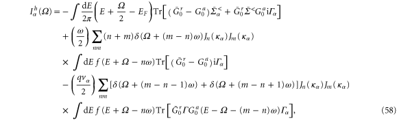
Performing the Fourier transformation on equations (21) and (22), the general frequency-dependent electric and heat currents are given by,

$$\begin{eqnarray*}\begin{array}{ccccccccccccccc} I_{\alpha }^{e}(\Omega ) & = & -q\int \frac{{\rm d}E}{2\pi }\int \frac{d{{E}^{\prime }}}{2\pi }{\rm Tr}\left[ {{G}^{r}}(E+\Omega ,{{E}^{\prime }})\Sigma _{\alpha }^{\lt }({{E}^{\prime }},E)+{{G}^{\lt }}(E+\Omega ,{{E}^{\prime }})\Sigma _{\alpha }^{a}({{E}^{\prime }},E) \right. \\ {} & {} & -\left. \Sigma _{\alpha }^{\lt }(E+\Omega ,{{E}^{\prime }}){{G}^{a}}({{E}^{\prime }},E)-\Sigma _{\alpha }^{r}(E+\Omega ,{{E}^{\prime }}){{G}^{\lt }}({{E}^{\prime }},E) \right] \\ \end{array}\end{eqnarray*}$$

$$\begin{eqnarray}\begin{array}{ccccccccccccccc} I_{\alpha }^{h}(\Omega ) & = & -\int \frac{{\rm d}E}{2\pi }\int \frac{d{{E}^{\prime }}}{2\pi }{\rm Tr}\left[ {{G}^{r}}(E+\Omega ,{{E}^{\prime }})\tilde{\Sigma }_{\alpha }^{\lt }({{E}^{\prime }},E)+{{G}^{\lt }}(E+\Omega ,{{E}^{\prime }})\tilde{\Sigma }_{\alpha }^{a}({{E}^{\prime }},E) \right. \\ {} & {} & -\left. \tilde{\Sigma }_{\alpha }^{\lt }(E+\Omega ,{{E}^{\prime }}){{G}^{a}}({{E}^{\prime }},E)-\tilde{\Sigma }_{\alpha }^{r}(E+\Omega ,{{E}^{\prime }}){{G}^{\lt }}({{E}^{\prime }},E) \right]. \\ \end{array}\end{eqnarray} \tag{ 23 }$$

It is straightforward to find,

$$\begin{eqnarray}&&\mathop{\sum }\limits_{\alpha }I_{\alpha }^{e}(\Omega )=q\Omega \int \frac{{\rm d}E}{2\pi }{\rm Tr}[{{G}^{\lt }}(E+\Omega ,E)]\end{eqnarray} \tag{ 24 }$$

which is the continuity equation for charge transport. Once the Poisson equation is solved, equations (8) and (24) lead to ${{\sum }_{\alpha }}I_{\alpha }^{e}(\Omega )=0,$ which is the current conservation. Obviously, if the Coulomb interaction U is not included in the Green's function, the current would not be conserved unless $\Omega =0$ (DC limit). The reason is that without the Coulomb interaction U the displacement current is left out, and the current we calculate is just the conduction current. It is the total current (conduction current plus displacement current) that is conserved.

In the linear regime, it has been shown in [4] that the Onsager relation holds

$$\begin{eqnarray}&&{{G}_{\alpha \beta }}(\Omega ,B)={{G}_{\beta \alpha }}(\Omega ,-B)\end{eqnarray} \tag{ 25 }$$

where ${{G}_{\alpha \beta }}$ is the frequency-dependent conductance. Now we show that for a multi-probe system, the Onsager relation together with the gauge-invariant condition leads to the current conservation automatically. The gauge-invariant condition with $-B$ means ${{\sum }_{\alpha }}{{G}_{\beta \alpha }}(-B)=0$ [4], which is equivalent to current conservation with B, ${{\sum }_{\alpha }}{{G}_{\alpha \beta }}(B)=0$, from the Onsager relation.

In the next subsection, we first discuss the DC limit of our formalism and discuss the gauge-invariant condition.

2.3. DC heat current

In the DC limit, the time translational symmetry is restored, and the two-time Green's function depends only on the time difference. Equation (22) can be written in energy space as follows

$$\begin{eqnarray}&&I_{\alpha }^{h}(t)=-\int \frac{{\rm d}E}{2\pi }{\rm Tr}[{{G}^{r}}(E)\tilde{\Sigma }_{\alpha }^{\lt }(E)+{{G}^{\lt }}(E)\tilde{\Sigma }_{\alpha }^{a}(E)-\tilde{\Sigma }_{\alpha }^{\lt }(E){{G}^{a}}(E)-\tilde{\Sigma }_{\alpha }^{r}(E){{G}^{\lt }}(E],\end{eqnarray} \tag{ 26 }$$

where the self-energy is obtained according to equation (20) with $\omega =0$. In this limit, equation (20) gives a δ function $\delta (\epsilon _{k\alpha }^{0}+q{{v}_{\alpha }}-E)$ after the Fourier transform. Finally we find

$$\begin{eqnarray}&&\tilde{\Sigma }_{\alpha }^{\gamma }(E)=(E-{{E}_{F}}-q{{v}_{\alpha }})\Sigma _{\alpha }^{\gamma }(E)\end{eqnarray} \tag{ 27 }$$

where $\Sigma _{\alpha }^{\gamma }(E)$ is the self-energy of the charge transport. Therefore, the DC heat current is given by [28, 29]

$$\begin{eqnarray}&&I_{\alpha }^{h}=\mathop{\sum }\limits_{\beta }\int (E-{{E}_{F}}-q{{v}_{\alpha }}){\rm Tr}[({{f}_{\alpha }}-{{f}_{\beta }}){{{\bf T}}_{\alpha \beta }}(E,U)]\frac{{\rm d}E}{2\pi }\end{eqnarray} \tag{ 28 }$$

where, ${{{\bf T}}_{\alpha \beta }}={{\Gamma }_{\alpha }}{{G}^{r}}{{\Gamma }_{\beta }}{{G}^{a}}$ is the transmission matrix.

We will show below that equation (28) is gauge invariant. To show the gauge invariance, we shift all the bias by a constant amount v₀, i.e., from ${{v}_{\alpha }}$ to ${{v}_{\alpha }}+{{v}_{0}}$. Keep in mind that we have included the self-consistent Coulomb potential U in the Hamiltonian, and U becomes $U+{{v}_{0}}$ after the shift. Since the self-energy ${{\Sigma }^{r}}(E)$ and Fermi distribution function depend on $E-q{{v}_{\alpha }},$ while the Green's function depends on $E-H-U-{{\Sigma }^{r}}(E)$, we can shift the dummy energy variable from E to $E+q{{v}_{0}}$. As a result, the heat current remains the same, which is the gauge-invariant condition.

To show the Onsager relation for the linear heat current, we will use the following relations when the external magnetic field is reversed [4]

$$\begin{eqnarray}\begin{array}{ccccccccccccccc} {{G}^{r,a}}(E,B) & = & {{[{{G}^{r,a}}(E,-B)]}^{T}} \\ {{\Gamma }_{\alpha }}(E,B) & = & {{[{{\Gamma }_{\alpha }}(E,-B)]}^{T}} \\ \end{array}\end{eqnarray} \tag{ 29 }$$

where the superscript T denotes the transpose, and ${{G}^{r,a}}$ and Γ are matrices in real space. Define the electrothermal admittance as

$$\begin{eqnarray*}&&G_{\alpha \beta }^{h}=q\int (E-{{E}_{F}})[-{{\partial }_{E}}f(E)]{\rm Tr}[{{{\bf T}}_{\alpha \beta }}]\frac{{\rm d}E}{2\pi }.\end{eqnarray*}$$

It is then straightforward to prove the Onsager relation

$$\begin{eqnarray}&&G_{\alpha \beta }^{h}(B)=G_{\beta \alpha }^{h}(-B).\end{eqnarray} \tag{ 30 }$$

In the next subsection, we study AC heat current at small bias. In the limit of the small bias, we can expand the expression of heat current to the linear and nonlinear order in terms of external bias to investigate the electrothermal admittance. In the following, a procedure on how to expand the heat current is presented using NEGF. The transport properties of the heat current in the presence of the Coulomb interaction will also be discussed.

2.4. Linear heat current

In the small bias limit, we can expand the Green's function ${{G}^{\gamma }}(t,{{t}_{1}})$ and self-energy $\tilde{\Sigma }_{\alpha }^{\gamma }(t,{{t}_{1}})$ up to the first order in terms of the bias ${{v}_{\alpha }}$ [30, 31].

$$\begin{eqnarray}&&{{G}^{\gamma }}(t,{{t}_{1}})=G_{0}^{\gamma }(t,{{t}_{1}})+g_{1}^{\gamma }(t,{{t}_{1}})\end{eqnarray} \tag{ 31 }$$

and

$$\begin{eqnarray}&&\tilde{\Sigma }_{\alpha }^{\gamma }(t,{{t}_{1}})=\tilde{\Sigma }_{\alpha 0}^{\gamma }(t,{{t}_{1}})+\tilde{\sigma }_{\alpha 1}^{\gamma }(t,{{t}_{1}})\end{eqnarray} \tag{ 32 }$$

where $G_{0}^{r}(t,{{t}_{1}})$ is the equilibrium Green's function and $g_{1}^{r}(t,{{t}_{1}})$ is the first-order correction. After substituting equations (31) and (32) into equation (22), the heat current $I_{\alpha 1}^{h}(t)$ in the linear response regime is easily obtained,

$$\begin{eqnarray}\begin{array}{ccccccccccccccc} I_{\alpha 1}^{h}(t) & = & -\int {\rm d}{{t}_{1}}{\rm Tr}\left[ G_{0}^{r}(t,{{t}_{1}})\tilde{\sigma }_{\alpha 1}^{\lt }({{t}_{1}},t)+g_{1}^{r}(t,{{t}_{1}})\tilde{\Sigma }_{\alpha 0}^{\lt }({{t}_{1}},t) \right. \\ {} & {} & +\left. G_{0}^{\lt }(t,{{t}_{1}})\tilde{\sigma }_{\alpha 1}^{a}({{t}_{1}},t)+g_{1}^{\lt }(t,{{t}_{1}})\tilde{\Sigma }_{\alpha 0}^{a}({{t}_{1}},t)+c.c. \right]. \\ \end{array}\end{eqnarray} \tag{ 33 }$$

Note that the quantities appearing in equation (33) with the subscript 0 like $G_{0}^{\gamma }(t,{{t}_{1}})$ and $\tilde{\Sigma }_{\alpha 0}^{\gamma }(t,{{t}_{1}})$ are all the equilibrium functions and only depend on the time difference $(t-{{t}_{1}}),$ while the other non-equilibrium quantities depend on the double-time indices t and ${{t}_{1}}.$ Taking the Fourier transform, the frequency-dependent linear heat current is

$$\begin{eqnarray*}\begin{array}{ccccccccccccccc} I_{\alpha 1}^{h}(\Omega ) & = & -\int \frac{{\rm d}E}{2\pi }{\rm Tr}\left[ G_{0}^{r}({{E}_{+}})\tilde{\sigma }_{\alpha 1}^{\lt }({{E}_{+}},E)+g_{1}^{r}({{E}_{+}},E)\tilde{\Sigma }_{\alpha 0}^{\lt }(E)+G_{0}^{\lt }({{E}_{+}})\tilde{\sigma }_{\alpha 1}^{a}({{E}_{+}},E) \right. \\ {} & {} & +g_{1}^{\lt }({{E}_{+}},E)\tilde{\Sigma }_{\alpha 0}^{a}(E)-\tilde{\sigma }_{\alpha 1}^{\lt }({{E}_{+}},E)G_{0}^{a}(E)-\tilde{\Sigma }_{\alpha 0}^{\lt }({{E}_{+}})g_{1}^{a}({{E}_{+}},E) \\ {} & {} & -\left. \tilde{\sigma }_{\alpha 1}^{r}({{E}_{+}},E)G_{0}^{\lt }(E)-\tilde{\Sigma }_{\alpha 0}^{r}(E)g_{1}^{\lt }({{E}_{+}},E) \right] \\ \end{array}\end{eqnarray*}$$

where ω is the driving frequency, Ω is the response frequency, and ${{E}_{+}}=E+\Omega$.

To further simplify the expression, we need to calculate the new quantity $\tilde{\Sigma }_{\alpha }^{\gamma }({{t}_{1}},t).$ Expanding equation (20) in powers of ${{v}_{\alpha }}$ and taking the Fourier transform, we find the 0th order and the first-order terms of $\tilde{\Sigma }_{\alpha }^{\gamma }({{E}_{+}},E)$

$$\begin{eqnarray*}&&\tilde{\Sigma }_{\alpha 0}^{\gamma }(E)=\Sigma _{0\alpha }^{\gamma }(E)(E-{{E}_{F}})\end{eqnarray*}$$

$$\begin{eqnarray*}&&\tilde{\sigma }_{\alpha 1}^{\gamma }({{E}_{+}},E)=\frac{q{{v}_{\alpha }}(\Omega )}{\Omega }[\tilde{\Sigma }_{0\alpha }^{\gamma }(E)-\tilde{\Sigma }_{0\alpha }^{\gamma }(E+\Omega )]\end{eqnarray*}$$

where ${{v}_{\alpha }}(\Omega )=\pi {{v}_{\alpha }}[\delta (\Omega +\omega )+\delta (\Omega -\omega )]$ and $\Sigma _{0\alpha }^{\gamma }(E)$ is the equilibrium self-energy.

The first-order correction of the retarded, advanced, and lesser Green's function $g_{1}^{r,a,\lt }$ has been calculated in reference [4]. Using the abbreviation $\ {{G}_{0}}(E)\equiv G,$ ${{G}_{0}}({{E}_{+}})\equiv \bar{G}$, $\bar{f}=f({{E}_{+}})$, and ${{g}_{1}}({{E}_{+}},E)\equiv \bar{g},$ etc., we have

$$\begin{eqnarray}&&\bar{g}_{1}^{r,a}={{\bar{G}}^{r,a}}(\bar{\sigma }_{1}^{r,a}+{{U}_{1}}){{G}^{r,a}}\end{eqnarray} \tag{ 34 }$$

$$\begin{eqnarray}&&\bar{g}_{1}^{\lt }={{\bar{G}}^{r}}\bar{\sigma }_{1}^{\lt }{{G}^{a}}+{{\overline{{{g}_{1}}}}^{r}}\Sigma _{0}^{\lt }{{G}^{a}}+{{\bar{G}}^{r}}\bar{\Sigma }_{0}^{\lt }\bar{g}_{1}^{a}\end{eqnarray} \tag{ 35 }$$

where ${{U}_{1}}(\Omega )=q{{\sum }_{\alpha }}{{u}_{\alpha }}(\Omega ){{v}_{\alpha }}(\Omega )$. In the wideband limit [32], the linewidth function is independent of the energy, and the equilibrium self-energy of the lead α is $\Sigma _{\alpha }^{r,a}=\mp i{{\Gamma }_{\alpha }}/2.$ In this approximation, we have

$$\begin{eqnarray}\begin{array}{ccccccccccccccc} \tilde{\sigma }_{\alpha 1}^{r,a}({{E}_{+}},E) & = & \pm {\rm i}q{{v}_{\alpha }}(\Omega )\frac{{{\Gamma }_{\alpha }}}{2} \\ \tilde{\sigma }_{\alpha 1}^{\lt }({{E}_{+}},E) & = & \;\frac{q{{v}_{\alpha }}(\Omega )}{\Omega }{\rm i}{{\Gamma }_{\alpha }}[(E-{{E}_{F}})f-({{E}_{+}}-{{E}_{F}})\bar{f}] \\ g_{1}^{r,a}({{E}_{+}},E) & = & {{{\bar{G}}}^{r,a}}{{U}_{1}}(\Omega ){{G}^{r,a}} \\ g_{1}^{\lt }({{E}_{+}},E) & = & \;{\rm i}q\mathop{\sum }\limits_{\alpha }\frac{f-\bar{f}}{\Omega }{{{\bar{G}}}^{r}}{{v}_{\alpha }}(\Omega ){{\Gamma }_{\alpha }}{{G}^{a}}+{\rm i}qf{{{\bar{G}}}^{r}}{{U}_{1}}{{G}^{r}}\Gamma {{G}^{a}}+{\rm i}q\bar{f}{{{\bar{G}}}^{r}}\Gamma {{{\bar{G}}}^{a}}{{U}_{1}}{{G}^{a}}. \\ \end{array}\end{eqnarray} \tag{ 36 }$$

Using equation (36) the linear frequency-dependent heat current becomes,

$$\begin{eqnarray}\begin{array}{ccccccccccccccc} I_{\alpha 1}^{h}(\Omega ) & = & -\int \frac{{\rm d}E}{2\pi }\frac{f-\bar{f}}{\Omega }(E+\frac{\Omega }{2}-{{E}_{F}}){\rm Tr}\left[ ({{{\bar{G}}}^{r}}-{{G}^{a}})q{{v}_{\alpha }}(\Omega ){\rm i}{{\Gamma }_{\alpha }}-{{{\bar{G}}}^{r}}\mathop{\sum }\limits_{\beta }q{{v}_{\beta }}(\Omega ){{\Gamma }_{\beta }}{{G}^{a}}{{\Gamma }_{\alpha }} \right. \\ {} & {} & +\left. \Omega {{{\bar{G}}}^{r}}{{U}_{1}}{{G}^{a}}{\rm i}{{\Gamma }_{\alpha }} \right]+\int \frac{{\rm d}E}{4\pi }(f-\bar{f}){\rm Tr}[({{G}^{a}}+{{{\bar{G}}}^{r}}){\rm i}{{\Gamma }_{\alpha }}(q{{v}_{\alpha }}(\Omega )-{{U}_{1}})], \\ \end{array}\end{eqnarray} \tag{ 37 }$$

where we have made the Thomas–Fermi approximation [3]. The first-order electrothermal admittance $G_{\alpha \beta }^{h}$ is defined similarly to the electric dynamic conductance [16]

$$\begin{eqnarray*}&&I_{\alpha 1}^{h}(\Omega )=\mathop{\sum }\limits_{\beta }G_{\alpha \beta }^{h}(\Omega ){{v}_{\beta }}(\Omega )\end{eqnarray*}$$

From equation (37) we find,

$$\begin{eqnarray}&&G_{\alpha \beta }^{h}(\Omega )=G_{\alpha \beta }^{h,(1)}(\Omega )+G_{\alpha \beta }^{h,(2)}(\Omega ),\end{eqnarray} \tag{ 38 }$$

where we have split electrothermal admittance into two parts: $G_{\alpha \beta }^{h,(1)}(\Omega ),$ which is related to the charge conductance $G_{\alpha \beta }^{e}(\Omega ),$ and $G_{\alpha \beta }^{h,(2)}(\Omega )$, defined as⁶

$$\begin{eqnarray}&&G_{\alpha \beta }^{h,(1)}(\Omega )=-q\int \frac{{\rm d}E}{2\pi }\frac{f-\bar{f}}{\Omega }(E+\frac{\Omega }{2}-{{E}_{F}}){\rm Tr}[{{g}_{\alpha \beta }}(\Omega ,E)],\end{eqnarray} \tag{ 39 }$$

and

$$\begin{eqnarray}&&G_{\alpha \beta }^{h,(2)}(\Omega )=q\int \frac{{\rm d}E}{4\pi }(f-\bar{f}){\rm Tr}[({{G}^{a}}+{{\bar{G}}^{r}}){\rm i}{{\Gamma }_{\alpha }}({{\delta }_{\alpha \beta }}-{{u}_{\beta }}(\Omega ))],\end{eqnarray} \tag{ 40 }$$

respectively, where we have introduced an energy-dependent local dynamic conductance matrix

$$\begin{eqnarray}&&{{g}_{\alpha \beta }}(\Omega ,E)=({{\bar{G}}^{r}}-{{G}^{a}}){\rm i}{{\Gamma }_{\beta }}{{\delta }_{\alpha \beta }}-{{\bar{G}}^{r}}{{\Gamma }_{\beta }}{{G}^{a}}{{\Gamma }_{\alpha }}+\Omega {{\bar{G}}^{r}}{{u}_{\beta }}(\Omega ){{G}^{a}}{\rm i}{{\Gamma }_{\alpha }},\end{eqnarray} \tag{ 41 }$$

which is related to the dynamic charge conductance

$$\begin{eqnarray}&&G_{\alpha \beta }^{e}(\Omega )=-{{q}^{2}}\int \frac{{\rm d}E}{2\pi }\frac{f-\bar{f}}{\Omega }{\rm Tr}[{{g}_{\alpha \beta }}(\Omega ,E)].\end{eqnarray} \tag{ 42 }$$

Here the characteristic potential ${{u}_{\alpha }}(\Omega )$ is used, which satisfies the Poisson-like equation [4]

$$\begin{eqnarray}&&{{\nabla }^{2}}{{u}_{\alpha }}(\Omega ,x)=-4\pi {{q}^{2}}\frac{{\rm d}{{n}_{\alpha }}(\Omega ,x)}{{\rm d}E}+4\pi {{q}^{2}}\frac{{\rm d}n(\Omega ,x)}{{\rm d}E}{{u}_{\alpha }}(\Omega ,x),\end{eqnarray} \tag{ 43 }$$

where we have introduced the frequency-dependent injectivity matrix

$$\begin{eqnarray}&&\frac{{\rm d}{{n}_{\alpha }}(\Omega )}{{\rm d}E}=\int \frac{{\rm d}E}{2\pi }\frac{f-\bar{f}}{\Omega }[{{\bar{G}}^{r}}{{\Gamma }_{\alpha }}{{G}^{a}}]\end{eqnarray} \tag{ 44 }$$

and the frequency-dependent emissivity matrix

$$\begin{eqnarray}&&\frac{{\rm d}{{{\bar{n}}}_{\alpha }}(\Omega )}{{\rm d}E}=\int \frac{{\rm d}E}{2\pi }\frac{f-\bar{f}}{\Omega }[{{G}^{a}}{{\Gamma }_{\alpha }}{{\bar{G}}^{r}}].\end{eqnarray} \tag{ 45 }$$

The boundary condition of the Poisson-like equation is that ${{u}_{\alpha }}$ deep inside α lead is 1 and is zero deep inside of other leads.

In this section, we examine the gauge-invariant electrothermal admittance and the departure of the Onsager relation for a linear dynamic heat current.

A gauge-invariant condition means that if we shift all voltages by a constant amount v₀, the heat current should not alter. This amounts to the condition ${{\sum }_{\beta }}G_{\alpha \beta }^{h}=0$. Since the dynamic charge current given in equation (42) satisfies the current conserving and gauge-invariant conditions, we have ${{\sum }_{\alpha }}G_{\alpha \beta }^{h,(1)}(\Omega )={{\sum }_{\beta }}G_{\alpha \beta }^{h,(1)}(\Omega )=0$. Using the sum rule for characteristic potential ${{\sum }_{\alpha }}{{u}_{\alpha }}=1$, we find from equation (40) ${{\sum }_{\beta }}G_{\alpha \beta }^{h,(2)}(\Omega )=0$. This shows that the gauge-invariant condition is satisfied for electrothermal admittance when the self-consistent Coulomb interaction is included.

Now we examine the Onsager relation for the electrothermal admittance. We note that in the AC regime, equation (29) is still valid, from which the Onsager relation has been shown to be valid for the dynamic conductance matrix [4]

$$\begin{eqnarray*}&&{\rm Tr}[{{g}_{\alpha \beta }}(\Omega ,E,B)]={\rm Tr}[{{g}_{\beta \alpha }}(\Omega ,E,-B)].\end{eqnarray*}$$

This shows that $G_{\alpha \beta }^{h,(1)}$ satisfies the Onsager relation⁷ ,

$$\begin{eqnarray}&&G_{\alpha \beta }^{h,(1)}(\Omega ,B)=G_{\beta \alpha }^{h,(1)}(\Omega ,-B).\end{eqnarray} \tag{ 46 }$$

However, for $G_{\alpha \beta }^{h,(2)}$ we have from equations (29) and (40)

$$\begin{eqnarray}&&G_{\alpha \beta }^{h,(2)}(\Omega ,-B)=q\int \frac{{\rm d}E}{4\pi }(f-\bar{f}){\rm Tr}[i({{\delta }_{\alpha \beta }}-u_{\beta }^{T}(\Omega ,-B)){{\Gamma }_{\alpha }}({{G}^{a}}+{{\bar{G}}^{r}})].\end{eqnarray} \tag{ 47 }$$

For a two-probe system, the Onsager relation requires that $G_{11}^{h,(2)}(\Omega ,-B)=G_{11}^{h,(2)}(\Omega ,B)$. This in turn requires ${{u}_{\beta }}(\Omega ,B)$ to be an even function of B. It has been shown in reference [4] that

$$\begin{eqnarray}&&\frac{{\rm d}{{n}_{\alpha }}(\Omega ,-B)}{{\rm d}E}=\frac{{\rm d}{{{\bar{n}}}_{\alpha }}(\Omega ,B)}{{\rm d}E}\end{eqnarray} \tag{ 48 }$$

and

$$\begin{eqnarray}&&\frac{{\rm d}n(\Omega ,-B)}{{\rm d}E}=\frac{{\rm d}\bar{n}(\Omega ,B)}{{\rm d}E}.\end{eqnarray} \tag{ 49 }$$

From equation (43) we see that ${{u}_{\beta }}(\Omega ,B)$ is not an even function of the magnetic field, which agrees with reference [2] at the zero-frequency limit. For a quantum dot with a single level with quasi-neutrality approximation, we have ${{G}^{r}}=1/(E-{{E}_{0}}+i\Gamma )$, from which we find ${{u}_{\alpha }}(\Omega )={{\Gamma }_{\alpha }}/\Gamma ,$ which is an even function of B. As a result, for this special case, the Onsager relation holds for $G_{\alpha \beta }^{h,(2)}(\Omega ),$ and hence, for $G_{\alpha \beta }^{h}(\Omega )$.

In the next subsection, we derive the general nonlinear expression of the heat current.

3.1. Nonlinear heat current

Now we calculate the general nonlinear heat current. To make the derivation simple, we only discuss the case where the Coulomb interaction is absent. From equation (20), using the relation ${\rm exp} (i{{\kappa }_{\alpha }}{\rm sin} x)={{\sum }_{n}}{{J}_{n}}({{\kappa }_{\alpha }}){\rm exp} (inx)$ with ${{\kappa }_{\alpha }}=q{{v}_{\alpha }}/\omega ,$ and J_n being the Bessel function, the heat self-energy can be found as

$$\begin{eqnarray}&&\tilde{\Sigma }_{\alpha }^{\gamma }({{t}_{1}},{{t}_{2}})=\mathop{\sum }\limits_{knm}(\epsilon _{k\alpha }^{0}-{{E}_{F}})\Sigma _{0k\alpha }^{\gamma }({{t}_{1}}-{{t}_{2}}){{J}_{n}}({{\kappa }_{\alpha }}){{J}_{m}}({{\kappa }_{\alpha }})\times {{{\rm e}}^{-{\rm i}n\omega {{t}_{1}}}}{{{\rm e}}^{{\rm i}m\omega {{t}_{2}}}}.\end{eqnarray} \tag{ 50 }$$

Taking the Fourier transform, we have

$$\begin{eqnarray}\begin{array}{ccccccccccccccc} \tilde{\Sigma }_{\alpha }^{\gamma }(E,E^{\prime} ) & = & \mathop{\sum }\limits_{knm}(E-n\omega -{{E}_{F}})\cdot \Sigma _{0k\alpha }^{\gamma }(E-n\omega )\times {{J}_{n}}({{\kappa }_{\alpha }}){{J}_{m}}({{\kappa }_{\alpha }}) \\ {} & {} & \times 2\pi \delta (E-E^{\prime} +(m-n)\omega ). \\ \end{array}\end{eqnarray} \tag{ 51 }$$

In contrast, the electric self-energy in the Fourier space

$$\begin{eqnarray}&&\Sigma _{\alpha }^{\gamma }(E,E^{\prime} )=\mathop{\sum }\limits_{knm}\Sigma _{0k\alpha }^{\gamma }(E-n\omega ){{J}_{n}}({{\kappa }_{\alpha }}){{J}_{m}}({{\kappa }_{\alpha }})\times 2\pi \delta (E-E^{\prime} +(m-n)\omega ).\end{eqnarray} \tag{ 52 }$$

In the wideband limit, where the equilibrium self-energy is $\Sigma _{0\alpha }^{r,a}=\mp i{{\Gamma }_{\alpha }}/2$ with ${{\Gamma }_{\alpha }}$ independent of energy, it is not difficult to see that ${{\tilde{\Sigma }}^{r,a}}$ is of tri-diagonal form in energy space:

$$\begin{eqnarray}&&\tilde{\Sigma }_{\alpha }^{r,a}(E,E^{\prime} )=7\pi \Sigma _{0\alpha }^{r,a}\left[ 2(E-{{E}_{F}})\cdot \delta (E-E^{\prime} )-q{{v}_{\alpha }}(\delta (E-E^{\prime} -\omega )+\delta (E-E^{\prime} +\omega )) \right],\end{eqnarray} \tag{ 53 }$$

where we have used the relation

$$\begin{eqnarray}&&\mathop{\sum }\limits_{n}{{J}_{n}}(x){{J}_{n+l}}(x)={{\delta }_{l,0}},\end{eqnarray} \tag{ 54 }$$

and

$$\begin{eqnarray}&&\mathop{\sum }\limits_{n}n{{J}_{n}}(x){{J}_{n+l}}(x)=\frac{x}{2}({{\delta }_{l+1,0}}+{{\delta }_{l-1,0}}).\end{eqnarray} \tag{ 55 }$$

The retarded Green's function can be calculated from the Dyson equation

$$\begin{eqnarray}&&{{G}^{r}}(E,E^{\prime} )=2\pi G_{0}^{r}(E)\delta (E-E^{\prime} ),\end{eqnarray} \tag{ 56 }$$

while the lesser Green's function can be obtained by the Keldysh equation

$$\begin{eqnarray}&&{{G}^{\lt }}(E,E^{\prime} )=G_{0}^{r}(E){{\Sigma }^{\lt }}(E,E^{\prime} )G_{0}^{a}(E^{\prime} ).\end{eqnarray} \tag{ 57 }$$

With the expressions of ${{G}^{\gamma }}(E,E^{\prime} )$ and ${{\tilde{\Sigma }}^{\gamma }}(E,E^{\prime} )$, we find the general nonlinear frequency-dependent heat current as follows

$$\begin{eqnarray}\begin{array}{ccccccccccccccc} I_{\alpha }^{h}(\Omega ) & = & -\int \frac{{\rm d}E}{2\pi }(E+\frac{\Omega }{2}-{{E}_{F}}){\rm Tr}\left[ (\bar{G}_{0}^{r}-G_{0}^{a})\bar{\Sigma }_{\alpha }^{\lt }+\bar{G}_{0}^{r}{{{\bar{\Sigma }}}^{\lt }}G_{0}^{a}{\rm i}{{\Gamma }_{\alpha }} \right] \\ {} & {} & +\left( \frac{\omega }{2} \right)\mathop{\sum }\limits_{nm}(n+m)\delta (\Omega +(m-n)\omega ){{J}_{n}}({{\kappa }_{\alpha }}){{J}_{m}}({{\kappa }_{\alpha }}) \\ {} & {} & \times \int {\rm d}E\;f(E+\Omega -n\omega ){\rm Tr}\left[ (\bar{G}_{0}^{r}-G_{0}^{a}){\rm i}{{\Gamma }_{\alpha }} \right] \\ {} & {} & -\left( \frac{q{{v}_{\alpha }}}{2} \right)\mathop{\sum }\limits_{nm}[\delta (\Omega +(m-n-1)\omega )+\delta (\Omega +(m-n+1)\omega )]{{J}_{n}}({{\kappa }_{\alpha }}){{J}_{m}}({{\kappa }_{\alpha }}) \\ {} & {} & \times \int {\rm d}E\;f(E+\Omega -n\omega ){\rm Tr}\left[ \bar{G}_{0}^{r}\Gamma G_{0}^{a}(E-\Omega -(m-n)\omega ){{\Gamma }_{\alpha }} \right], \\ \end{array}\end{eqnarray} \tag{ 58 }$$

where $\bar{\Sigma }_{\alpha }^{\lt }$ is an abbreviation for $\Sigma _{\alpha }^{\lt }(E+\Omega ,E),$ defined in equation (52).

It should be noted that the first term of this equation is similar to the general formulae of electric current, except for an extra factor of $(E+\frac{\Omega }{2}-{{E}_{F}})$. The second and third term are written as an expansion of Bessel functions, which contribute to both linear and non-linear behaviors of the heat current in voltage and frequency. To compare with our result in the linear regime, we expand equation (58) in powers of ${{v}_{\alpha }}$. It is easy to show that the result recovers equation (37).

3.2. First-principles calculation

Before we end this section, we will discuss how to perform first-principles calculation of electrothermal admittance within the NEGF-DFT framework. We start with a mean field Hamiltonian for a particular nano-device by performing an equilibrium first-principle calculation to obtain-equilibrium Hamiltonian, including equilibrium charge density and Hartree potential U_eq [21]. After that, we construct the equilibrium Green's function, defined as

$$\begin{eqnarray}&&{{G}^{r}}=1/[E-H-{{U}_{eq}}-{{V}_{xc}}-{{\Sigma }^{r}}]\end{eqnarray} \tag{ 59 }$$

where U is the self-consistent Coulomb potential and V_xc is the potential due to exchange and correlation, which is the functional of charge density. If the non-orthogonal basis set is used, we have to replace E by ES in the above equation where S is the overlap matrix for the basis set. We then calculate the frequency-dependent local density of state ${\rm d}{{n}_{\alpha }}(\Omega ,x)/{\rm d}E$ defined in equation (44) and solve the Poisson-like equation (62) given below to find the frequency-dependent characteristic potential ${{u}_{\alpha }}(\Omega ,x)$ due to the AC bias. The boundary condition of Poisson-like condition is: u_L is zero deep inside of the right lead and is one deep inside of the left lead for two probe structures. Once the characteristic potential is found, the electrothermal admittance can be obtained from equation (38) and (39), and modified (40) described below.

For first principles, calculation, due to the presence of the exchange correlation potential, the Poisson-like equation (43) and electrothermal admittance (39) and (40) have to be modified. This is because the Dyson equation (9) has one more term,

$$\begin{eqnarray}&&{{G}^{r}}=G_{0}^{r}+{{G}^{r}}UG_{0}^{r}+{{G}^{r}}{{V}_{xc}}G_{0}^{r}+{{G}^{r}}{{\Sigma }^{r}}G_{0}^{r}\end{eqnarray} \tag{ 60 }$$

where

$$\begin{eqnarray}&&{{V}_{xc}}={{V}_{xc,eq}}+\mathop{\sum }\limits_{\alpha }{{v}_{xc,\alpha }}{{v}_{\alpha }}\end{eqnarray} \tag{ 61 }$$

and ${{v}_{xc,\alpha }}$ is the first-order correction to the equilibrium exchange correlation potential. We emphasize that since V_xc is a functional of charge density, and linear charge density is given by the right-hand side of equation (43), hence ${{v}_{xc,\alpha }}=w(\Omega ,x)[{\rm d}{{n}_{\alpha }}(\Omega ,x)/{\rm d}E-{\rm d}n(\Omega ,x)/{\rm d}E\;{{u}_{\alpha }}(\Omega ,x)]$ where $w(\Omega ,x)$ can be obtained, depending on the choice of exchange and correlation potential. Then the Poisson like equation becomes,

$$\begin{eqnarray}&&{{\nabla }^{2}}{{u}_{\alpha }}(\Omega )=-4\pi {{q}^{2}}\frac{{\rm d}{{n}_{\alpha }}(\Omega )}{{\rm d}E}+4\pi {{q}^{2}}\frac{{\rm d}n(\Omega )}{{\rm d}E}({{u}_{\alpha }}(\Omega )+{{v}_{xc,\alpha }}(\Omega )).\end{eqnarray} \tag{ 62 }$$

Finally we have to modify equation (40) by replacing ${{u}_{\alpha }}$ with ${{u}_{\alpha }}+{{v}_{xc,\alpha }}$.

In this section, we apply our theory to a nano capacitor and calculate the electrothermal admittance. As we mentioned in the introduction, Lim et al [16] has investigated the dynamic thermoelectric and heat current for a mesoscopic capacitor similar to the experimental setup of reference [33]. In this setup, a quantum dot system is capacitively coupled to a macroscopic metal, forming a capacitor. In this system, only density of states of the quantum dot contributes to the quantum admittance. The dynamic response of this quantum capacitor can be characterized by three parameters at low frequencies: a static electrochemical capacitance, a charge relaxation resistance, and a quantum inductance [34]. For this system, thermoelectric capacitance is found to be proportional to the derivative of density of states of the quantum dot, which can be tuned by gate voltage, giving rise to a different response (capacitive-like or inductive-like) to the external time-dependent temperature bias [16]. In addition, thermoelectric relaxation resistance is found to be non-universal, depending on sample details.

We consider a parallel plate nano capacitor, which consists of an insulator sandwiched by two nanoscale metallic plates called regions I and II (see figure 1). Due to the finite density of states of metallic plates; the potential is not fully screened. As a result, the electrochemical potential of the reservoir ${{V}_{\alpha }}$ ($\alpha =L,R$) is not equal to the electrostatic potential U_k ($k=I,II$) of the metallic plate, giving rise to a quantum correction to the capacitance, which has been confirmed experimentally [35]. We will first discuss how to obtain the electrochemical capacitance using the discrete potential model [36] and then use the same method to calculate the linear AC heat current.

For an applied bias ${{v}_{L}}\lt {{v}_{R}}$, we have an electron injected into region I with total charge Q_I. Due to the Coulomb interaction, a charge Q_II will be induced in both regions I and II. In general, the charge consists of an injected and induced charge, ${{Q}_{I}}={{Q}_{inj,I}}+{{Q}_{ind,I}}$. Here the injected charge is given by ${{Q}_{inj,I}}={{{\rm e}}^{2}}{{D}_{I}}{{v}_{L}},$ where D_I is the density of states in region I. The induced charge is related to Lindhard function [3]. If we use the Thomas–Fermi approximation, the result is much simpler: ${{Q}_{ind,I}}=-{{{\rm e}}^{2}}{{D}_{I}}{{U}_{I}}$ [36]. Therefore, we have

$$\begin{eqnarray}&&{{Q}_{I}}={{{\rm e}}^{2}}{{D}_{I}}({{v}_{L}}-{{U}_{I}}).\end{eqnarray} \tag{ 63 }$$

Similar expressions hold for the charge in region II. From the definition of classical capacitance denoted as C₀ and electrochemical capacitance denoted as ${{C}_{\mu }}$, we have [36]

$$\begin{eqnarray}&&{{Q}_{I}}={{C}_{0}}({{U}_{I}}-{{U}_{II}})\end{eqnarray} \tag{ 64 }$$

and

$$\begin{eqnarray}&&{{Q}_{I}}={{C}_{\mu }}({{v}_{L}}-{{v}_{R}}).\end{eqnarray} \tag{ 65 }$$

From equations (63), (64), and (65), we find

$$\begin{eqnarray}&&{{U}_{I}}={{v}_{L}}-\frac{{{C}_{\mu }}({{v}_{L}}-{{v}_{R}})}{{{{\rm e}}^{2}}{{D}_{I}}}\end{eqnarray} \tag{ 66 }$$

and

$$\begin{eqnarray}&&{{U}_{II}}={{v}_{R}}+\frac{{{C}_{\mu }}({{v}_{L}}-{{v}_{R}})}{{{{\rm e}}^{2}}{{D}_{II}}}.\end{eqnarray} \tag{ 67 }$$

Taking the difference between equations (66) and (67), we have

$$\begin{eqnarray}&&{{U}_{I}}-{{U}_{II}}={{v}_{L}}-{{v}_{R}}-{{C}_{\mu }}({{v}_{L}}-{{v}_{R}})(\frac{1}{{{{\rm e}}^{2}}{{D}_{I}}}+\frac{1}{{{{\rm e}}^{2}}{{D}_{II}}}).\end{eqnarray} \tag{ 68 }$$

Noting that ${{U}_{I}}-{{U}_{II}}=({{C}_{\mu }}/{{C}_{0}})({{v}_{L}}-{{v}_{R}})$, we finally arrive at

$$\begin{eqnarray}&&\frac{1}{{{C}_{\mu }}}=\frac{1}{{{C}_{0}}}+\frac{1}{{{{\rm e}}^{2}}{{D}_{I}}}+\frac{1}{{{{\rm e}}^{2}}{{D}_{II}}}\end{eqnarray} \tag{ 69 }$$

which was first obtained by Buttiker 20 years ago [3]. Clearly for a macroscopic sample with a large density of states, the quantum correction vanishes, and electrochemical capacitance reduces to classical capacitance. For the nanocapacitor, the low frequency dynamic charge conductance is given by ${{G}_{\alpha \beta }}(\Omega )=-{\rm i}{{{\rm e}}^{2}}\Omega {{C}_{\alpha \beta }}$ with ${{C}_{LR}}={{C}_{\mu }}$, ${{\sum }_{\alpha }}{{C}_{\alpha \beta }}=0,$ and ${{\sum }_{\beta }}{{C}_{\alpha \beta }}=0$ [3, 37].

Zoom In Zoom Out Reset image size

Now we examine the electrothermal admittance at low frequencies. We expand equations (39) and (40) to the first order in frequency at zero temperature and find ($q=-e$)⁸

$$\begin{eqnarray}&&I_{\alpha }^{h}=-\frac{{\rm ie}\Omega }{4\pi }\mathop{\sum }\limits_{\beta }{\rm Tr}({{G}^{a}}+{{G}^{r}}){{\Gamma }_{\alpha }}({{\delta }_{\alpha \beta }}-{{u}_{\beta }}){{v}_{\beta }}.\end{eqnarray} \tag{ 70 }$$

Since our theory is gauge invariant, we can choose ${{v}_{L}}=v$ and v_R = 0. In the discrete potential model, only two regions are considered; hence, the above equation becomes

$$\begin{eqnarray}\begin{array}{ccccccccccccccc} I_{L}^{h} & = & -\frac{{\rm ie}\Omega }{2\pi }{\rm Im}({{S}_{LL}}){{U}_{II}} \\ I_{R}^{h} & = & \frac{{\rm ie}\Omega }{2\pi }{\rm Im}({{S}_{RR}}){{U}_{I}} \\ \end{array}\end{eqnarray} \tag{ 71 }$$

where ${{S}_{\alpha \beta }}$ is the scattering matrix, and we have used the Fisher–Lee relation

$$\begin{eqnarray}&&{{S}_{\alpha \alpha }}=-1+{\rm iTr}({{G}^{r}}{{\Gamma }_{\alpha }}).\end{eqnarray} \tag{ 72 }$$

Using equations (66) and (67), we finally have

$$\begin{eqnarray}\begin{array}{ccccccccccccccc} I_{L}^{h} & = & -\frac{{\rm ie}\Omega }{2\pi }{\rm Im}({{S}_{LL}})\frac{{{C}_{\mu }}}{{{{\rm e}}^{2}}{{D}_{II}}}({{v}_{L}}-{{v}_{R}}) \\ I_{R}^{h} & = & \frac{{\rm ie}\Omega }{2\pi }{\rm Im}({{S}_{RR}})(1-\frac{{{C}_{\mu }}}{{{{\rm e}}^{2}}{{D}_{I}}})({{v}_{L}}-{{v}_{R}}) \\ \end{array}\end{eqnarray} \tag{ 73 }$$

where we have used the fact that the heat current is gauge invariant. The first-order term in frequency given in the above equation reflects the phase difference between bias voltage and heat current. We see that the heat current for the left or right lead may have a different phase, depending on the density of states of the lead as well as the phase of the scattering matrix. For a symmetric two-probe nano capacitor, we have ${{S}_{LL}}={{S}_{RR}}=-i{\rm exp} (i\phi )$ where ϕ is the phase accumulated in the scattering event [38]. Hence for a simple parallel-plate symmetric nano capacitor, we have $\phi =0$ and

$$\begin{eqnarray}&&I_{L}^{h}=-\frac{{\rm ie}\Omega }{2\pi }\frac{{{C}_{\mu }}}{{{{\rm e}}^{2}}{{D}_{II}}}({{v}_{L}}-{{v}_{R}}).\end{eqnarray} \tag{ 74 }$$

This is a typical capacitance-like behavior where the voltage lags behind the heat current. According to the convention of heat current, current flowing into the system is positive. Because of this and the fact that $1-{{C}_{\mu }}/{{{\rm e}}^{2}}{{D}_{I}}={{C}_{\mu }}/{{C}_{0}}+{{C}_{\mu }}/{{{\rm e}}^{2}}{{D}_{II}}$ is positive definite, we find that I^h_R show similar capacitance-like behavior. For a macroscopic capacitor, DOS can be treated as infinity. In this case, ${{C}_{\mu }}$ reduces to the classical capacitance C₀, and $I_{L}^{h}=0$ (up to the first order in frequency). This means that the heat current of the left lead follows the voltage instantly, while the voltage still lags behind the heat current of the right lead.

Finally, adding up the total heat current, we have

$$\begin{eqnarray}&&I_{L}^{h}+I_{R}^{h}=\frac{{\rm ie}\Omega }{2\pi }\frac{{{C}_{\mu }}}{{{C}_{0}}}({{v}_{L}}-{{v}_{R}}).\end{eqnarray} \tag{ 75 }$$

In summary, we have developed the general expression for linear heat current in AC regime. By including the self-consistent Coulomb interaction, this theory is shown to be gauge invariant. The departure of the Onsager relation is observed for electrothermal admittance. We have also discussed possible extension of this formalism to the case of first-principles calculation. We have applied our theory to a nanocapacitor, where the self-consistent Coulomb interaction is essential for the electrochemical capacitance. A general expression has been obtained for heat current in terms of electrochemical capacitance and the scattering matrix element, up to the first order in frequency.

This work was financially supported by the University Grant Council (Contract No. AoE/P-04/08) of the Government of HKSAR and the National Natural Science Foundation of China (Grant No. 11374246).